

Abstract
Evapotranspiration (ET), as a key exchanging component of the land energy, water and carbon cycles, is expected to increase in response to greening land under a warming climate. However, the relative importance of major drivers (e.g. leaf area index (LAI), climate forcing, atmospheric CO2, etc) to long-term ET change remain largely unclear. Focusing on the Eurasia which experienced the strong vegetational greening, we aim to estimate the long-term ET trend and its drivers' relative contributions by applying a remote sensing-based water-carbon coupling model— Penman–Monteith–Leuning version 2 (PML-V2) driven by observational climate forcing and CO2 records, and satellite-based LAI, albedo and emissivity. The PML-V2 estimated an increasing ET trend (6.20 ± 1.13 mm year−1 decade−1, p < 0.01) over Eurasia during 1982–2014, which is close to the ensemble mean (6.51 ± 3.10 mm year−1 decade−1) from other three ET products (GLEAMv3.3a, ERA5 and CRv1.0). The PML-based ET overall agrees well with water-balance derived ET in detecting the trend directions. We find that the Eurasian ET increasing trend was mostly from vegetated regions over central and eastern Europe, Indian and southeast China where ET trends were larger than 20 mm year−1 decade−1. Modeling sensitivity experiments indicate that the Eurasian ET trend was mainly dominated by positive contributions from climate forcing change (40%) and increased LAI (22%), but largely offset by a negative contribution of increased CO2 (26%). Our results highlight the importance of the suppression effect of increasing CO2-induced stomatal closure on transpiration. This effect was rarely considered in diagnostic ET products but plays a key role to ensure that the long-term ET trend should not be overestimated by only accounting for greening-induced increases in transpiration and rainfall interception.
Export citation and abstract BibTeX RIS

Original content from this work may be used under the terms of the Creative Commons Attribution 4.0 license. Any further distribution of this work must maintain attribution to the author(s) and the title of the work, journal citation and DOI.
1. Introduction
The greenhouse effects of increasing concentrations of atmospheric CO2 and other greenhouse gases have induced global warming and related environmental changes (e.g. radiation, precipitation and wind) which are expected to increase evapotranspiration (ET) (Jung et al 2010, Zhang et al 2012, 2016, Ma et al 2020, Pascolini-Campbell et al 2021) and substantially modify the global water cycle (Milly et al 2005, Gedney et al 2006, Huntington 2006, Betts et al 2007, Wang et al 2018, Mankin et al 2019). However, long-term ET changes are highly uncertain, largely due to the poor understanding of the underlying mechanism and relative importance from surface driving variables and the uncertainties of different forcing sources and approaches (Zhang et al 2017, Lian et al 2021, Pascolini-Campbell et al 2021).
Since 1980s, satellite-based observations have revealed continuous vegetation greening trends (measured by leaf area index (LAI) in this study) over Eurasia, which are attributed to the combined effect from increased CO2 fertilization effect, climate forcing change, land use change, and nitrogen deposition (Norby and Zak 2011, Zhu et al
2016, Chen et al
2019). The increased LAI is expected to increase canopy transpiration ( ) and evaporation from vegetation intercepted precipitation (
 ), but may reduce bare soil evaporation (
 ) due to lower solar radiation from larger vegetation coverage (Zhang et al
2015, 2016, Lemordant et al
2018, Zeng et al
2018). Meanwhile, increased CO2 also induced the suppression effect on plant/canopy transpiration (
) due to lower solar radiation from larger vegetation coverage (Zhang et al
2015, 2016, Lemordant et al
2018, Zeng et al
2018). Meanwhile, increased CO2 also induced the suppression effect on plant/canopy transpiration ( ) by reducing leaf stomatal conductance which regulates exchanges of both CO2 and H2O molecules between the plant and the atmosphere (Field et al
1995, Katul et al
2009, Damour et al
2010, Milly and Dunne 2016, Swann et al
2016), thereby may partly offset the LAI-induced changes in ET. Just as importantly, variations in terrestrial ET are largely controlled by surface climate forcing which is reflected by atmospheric water demand, surface available energy, soil water supply, and feedbacks between atmosphere, vegetation and soil (e.g. Milly and Dunne 2002, Teuling et al
2009, Jung et al
2010, Wang and Dickinson 2012, Hoek van Dijke et al
2020). Overall, as the major external drivers of terrestrial ET or its components, the LAI, CO2 and climate forcing over the last decades may have had strongly modified the long-term changes in ET over Eurasia. However, the relative contributions of these major external drivers to the long-term trend in Eurasian ET since 1980s remain poorly understood.
) by reducing leaf stomatal conductance which regulates exchanges of both CO2 and H2O molecules between the plant and the atmosphere (Field et al
1995, Katul et al
2009, Damour et al
2010, Milly and Dunne 2016, Swann et al
2016), thereby may partly offset the LAI-induced changes in ET. Just as importantly, variations in terrestrial ET are largely controlled by surface climate forcing which is reflected by atmospheric water demand, surface available energy, soil water supply, and feedbacks between atmosphere, vegetation and soil (e.g. Milly and Dunne 2002, Teuling et al
2009, Jung et al
2010, Wang and Dickinson 2012, Hoek van Dijke et al
2020). Overall, as the major external drivers of terrestrial ET or its components, the LAI, CO2 and climate forcing over the last decades may have had strongly modified the long-term changes in ET over Eurasia. However, the relative contributions of these major external drivers to the long-term trend in Eurasian ET since 1980s remain poorly understood.
In this study, using a new version of the three-layer remote sensing-based ET model PML-V2 (Zhang et al 2019) that considers the combined impact from the major external drivers (i.e. LAI, CO2, climate forcing, etc) on the simulation of ET, we aim to (a) provide an observation-constrained estimation of historical ET over Eurasia, (b) identify regional dominant drivers of the long-term trends in annual ET over Eurasia, and (c) quantify the relative contributions of the major external drivers (i.e. LAI, CO2, climate forcing, etc) to the ET trends by using a group of modeling sensitivity experiments.
2. Materials and methods
2.1. Satellite data-driven ET model—PML-V2
The Penman–Monteith–Leuning model version 2 (PML-V2) was developed by coupling the widely-used photosynthesis model (Farquhar et al 1980) and a canopy stomatal conductance model (Yu et al 2004) with the Penman–Monteith energy balance equation (Monteith 1965) to jointly estimate GPP and ET (Leuning et al 2008, Zhang et al 2010b, 2016, 2019, Gan et al 2018). We used the PML-V2 for this study is due to that the PML-V2 model shows good performances for considering both effects from rising CO2, and increasing LAI and climate forcings on ET estimation, compared to the older version PML-V1 or other ET models, e.g. Global Land Evaporation Amsterdam Model (GLEAM) that did not consider rising CO2's impact on canopy stomatal conductance. The PML-V2 model has been applied to successfully produce the MODIS LAI-based global GPP and ET products at a 500 m and 8 d resolution since 2002, which were noticeably better than most widely used diagnostic GPP and ET products (Zhang et al 2019).
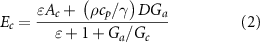
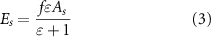
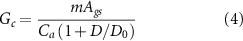
The PML-V2 model consists of three components for separately calculating the ET's three components (equations (1)–(3)): canopy transpiration ( ), soil evaporation (
 ) and rainfall interception (
 ),
),

The PML-V2 model simulates  (see supplementary text) based on a revised Gash-model scheme (van Dijk and Bruijnzeel 2001) with key parameters (see table S1 (available online at stacks.iop.org/ERL/16/124008/mmedia)) calibrated using filed measurements. The canopy transpiration (
 ) is estimated using the Penman–Monteith energy balance equation but the canopy stomatal conductance (
 ) is not a constant and changes with vegetational dynamics (equations (2) and (4)) through coupling with the photosynthesis process (
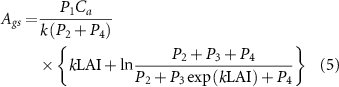
 ). The photosynthesis process (
 ) changes with increasing CO2 and LAI across different vegetation types, and then produces
  (equations (4)–(6)) and GPP (see supplementary text). The soil evaporation (
 ) depends on absorbed energy flux and soil water deficit,
where the surface available energy ( ) is divided into canopy absorbed energy (
 ) and soil absorbed energy (
 ),
),  and
and  ,
,  ,
,  ;
;  is the net radiation and
  is the ground heat flux (W m−2).
  , and
, and  is the slope of the curve relating saturation water vapor pressure to temperature (kPa °C−1).
  is the density of air (g m−3);
  is the specific heat of air at constant pressure (J g−1 °C−1);
  is vapor pressure deficit (kPa).
  is the aerodynamic conductance (m s−1);
  is the canopy conductance (m s−1);
  is a dimensionless variable that determines the water availability for soil evaporation, which is a fraction function of the accumulated precipitation and soil equilibrium evaporation for each grid cell (Zhang et al
2019).
is a dimensionless variable that determines the water availability for soil evaporation, which is a fraction function of the accumulated precipitation and soil equilibrium evaporation for each grid cell (Zhang et al
2019).
In PML-V2 model, the canopy stomatal conductance ( ) are calculated by the photosynthesis process (
 ) for each plant functional type (PFT) with the constraint of vapor pressure deficit (
 ) at surface,
where  ,
,  ,
,  ,
,  , and
, and  .
.  is the photosynthetically active radiation (PAR, in mol) from shortwave downward radiation.
  is the atmospheric CO2 concentration (in ppm or mol/mol).
  ,
,  ,
,  ,
,  are key parameters for photosynthesis process, i.e. maximum photosynthetic carboxylation efficiency (
 ), initial photochemical efficiency (
 ), initial value of the slope of CO2 response curve (
 ), and stomatal conductance coefficient (
 ), and Dmin, Dmax,
  are parameters to identify the constraint of atmospheric vapor pressure deficit in PML-V2 model (see table S1). All values of these key parameters for global ten major PFTs in table S1 were calibrated using half-monthly GPP, ET and climate forcing over 2002–2014 derived from 95 eddy covariance (EC) flux sites of the FLUXNET2015 dataset and AVHRR GIMMS3g-based LAI. The PFTs are defined from the NASA MCD12Q1 IGBP land cover classes (Friedl et al
2010). The detailed calibration method has been shown in Zhang et al (2019), which optimize the key parameters for each PFT by minimizing the objective function (F):
are parameters to identify the constraint of atmospheric vapor pressure deficit in PML-V2 model (see table S1). All values of these key parameters for global ten major PFTs in table S1 were calibrated using half-monthly GPP, ET and climate forcing over 2002–2014 derived from 95 eddy covariance (EC) flux sites of the FLUXNET2015 dataset and AVHRR GIMMS3g-based LAI. The PFTs are defined from the NASA MCD12Q1 IGBP land cover classes (Friedl et al
2010). The detailed calibration method has been shown in Zhang et al (2019), which optimize the key parameters for each PFT by minimizing the objective function (F):  , where
  and
and  are the Nash–Sutcliffe Efficiency (NSE) for ET and GPP, respectively, which are obtained by comparing the PML-V2 simulations and FLUXNET2015-based observations.
Using the parameter-calibrated PML-V2 model, we estimated grid cell-scale half-month ET and GPP using observational climate forcing, AVHRR GIMMS3g-based LAI and CO2 data, and compare them to observations at 95 eddy flux sites from FLUXNET2015-based dataset (figure S1). We show that compared to the FLUXNET2015-based observations, the PML-V2 model presents a good model performance with e.g. a NSE of 0.70, a root mean square error (RMSE) of 0.7, and a bias of −0.21% for half-month ET; and a NSE of 0.74, a RMSE of 2.05, and a bias of 3.8% for half-month GPP (figures S1(a) and (b)). Even under the cross-validation mode of the PML-V2 model, the comparing results are only slightly degraded, e.g. the NSE becomes 0.6 for ET and 0.61 for GPP (figures S1(c) and (d)).
2.2. Observational forcing datasets for estimating ET
In this study, we applied the PML-V2 model to produce historical coupled estimates of GPP, ET and its components  ,
,  and
and  over 1982–2014 at 0.05° and half-monthly resolutions. The forcing inputs for the PML-V2 model are land surface climate variables (i.e. precipitation, near-surface air temperature, pressure and relative humidity, wind speed at a 10 m height, downward longwave and shortwave radiations) from the GLDAS V2.0 observational 3 h 0.25° climate dataset (Rodell et al
2004, Beaudoing and Rodell 2019), the global satellite-based half-monthly LAI from the satellite AVHRR GIMMS3g V3 product (Zhu et al
2013), and the global satellite-based 8 d surface albedo for shortwave and surface emissivity for longwave radiation from the GLASS V4 product (Liu et al
2013, Cheng and Liang 2014). Atmospheric CO2 concentration data are provided by NOAA global monthly mean atmospheric CO2 records (ftp://aftp. cmdl.noaa.gov/products/trends/co2/co2_mm_gl.txt).
over 1982–2014 at 0.05° and half-monthly resolutions. The forcing inputs for the PML-V2 model are land surface climate variables (i.e. precipitation, near-surface air temperature, pressure and relative humidity, wind speed at a 10 m height, downward longwave and shortwave radiations) from the GLDAS V2.0 observational 3 h 0.25° climate dataset (Rodell et al
2004, Beaudoing and Rodell 2019), the global satellite-based half-monthly LAI from the satellite AVHRR GIMMS3g V3 product (Zhu et al
2013), and the global satellite-based 8 d surface albedo for shortwave and surface emissivity for longwave radiation from the GLASS V4 product (Liu et al
2013, Cheng and Liang 2014). Atmospheric CO2 concentration data are provided by NOAA global monthly mean atmospheric CO2 records (ftp://aftp. cmdl.noaa.gov/products/trends/co2/co2_mm_gl.txt).
2.3. Modeling sensitivity experiments for isolating driver contribution
To isolate individual environmental drivers' contribution to historical changes in ET,  ,
,  and
and  , we designed a group of modeling sensitivity experiments (see table 1) that are similar to those used in the Multi-Scale synthesis and Terrestrial Model Intercomparison Project (Huntzinger et al
2013). Using the PML-V2 model driven by observational climate forcing, observed atmospheric CO2, satellite-derived LAI, and albedo and emissivity datasets, we conducted five scenarios of sensitivity simulations (S1–S5, see table 1) by setting all drivers change with time (S1), or one or more drivers using fixed climate at 1982 (constant-1982) with others dynamic (S2–S4), or all constant-1982 drivers (S5 as the control run) as inputs over 1982–2014. Therefore, differences between pairs of these sensitivity simulations allow for a robust assessment of model-derived carbon and water fluxes (e.g. ET) sensitivity (including variability and trend) to individual drivers (S1 and S2 for albedo and emissivity's contribution (equation (7)), S2 and S3 for LAI's contribution (equation (8)), S3 and S4 for CO2's contribution (equation (9)) and S4 and S5 for climate's contribution (equation (10))),
, we designed a group of modeling sensitivity experiments (see table 1) that are similar to those used in the Multi-Scale synthesis and Terrestrial Model Intercomparison Project (Huntzinger et al
2013). Using the PML-V2 model driven by observational climate forcing, observed atmospheric CO2, satellite-derived LAI, and albedo and emissivity datasets, we conducted five scenarios of sensitivity simulations (S1–S5, see table 1) by setting all drivers change with time (S1), or one or more drivers using fixed climate at 1982 (constant-1982) with others dynamic (S2–S4), or all constant-1982 drivers (S5 as the control run) as inputs over 1982–2014. Therefore, differences between pairs of these sensitivity simulations allow for a robust assessment of model-derived carbon and water fluxes (e.g. ET) sensitivity (including variability and trend) to individual drivers (S1 and S2 for albedo and emissivity's contribution (equation (7)), S2 and S3 for LAI's contribution (equation (8)), S3 and S4 for CO2's contribution (equation (9)) and S4 and S5 for climate's contribution (equation (10))),


Table 1. Design of modeling sensitivity experiment for isolating driver contribution.
| Simulation scenarios (1982–2014) | |||||
|---|---|---|---|---|---|
| Model driver | S1 | S2 | S3 | S4 | S5 |
| Climate forcing | Dynamic | Dynamic | Dynamic | Dynamic | Constant |
| LAI | Constant | ||||
| CO2 | Constant | ||||
| Albedo and emissivity | Constant | ||||
Interactions between two or more drivers (S2−S4 for LAI and CO2's contribution, S3−S5 for climate and CO2's contribution, S2−S5 for LAI and CO2 and climate's contribution) can also be estimated. In this study, we estimated the overall interaction that is calculated by difference between the historical change (S1−S5) and the sum of individual driver's direct contribution (equations (7)–(10)). It is noted that we did not separate variables of climate forcing and therefore make our modeling sensitivity experiments smaller and results easy to interpret.
We calculated the relative contributions of individual drivers (table 1) to the global or regional long-term changes or trends in the studying variables (e.g. annual ET) by
where  is one of the four major model drivers (climate change, CO2, LAI, surface albedo and emissivity), and
  is a response variable (e.g. ET,
  ,
,  or
or  ). Equation (11) indicates that a negative (positive) value of the relative contribution of
  means that driver
  has a negative (positive) contribution to the overall change or trend in the response variable
  . Therefore, the overall contribution should be summed from all absolute values of individual relative contributions (i.e.
  ) to be sure that the summed result is 100%.
2.4. Datasets for validation and comparison
2.4.1. Observational annual ET derived from basin-scale water balance
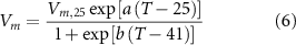
At a large scale (e.g. basin-scale in this study), the ET can be easily estimated by the water-balance method, considered as the difference between precipitation (P) and basin streamflow (Q) and change in water storage (ΔS), that is, ETwb = P − Q − ΔS. For a given basin, P and Q are observed from meteorological or hydrological stations, and ΔS has been widely estimated from the gravity recovery and climate experiment (GRACE) satellite-based gravity field. Therefore, the derived ETwb is often regarded as 'observational' to evaluate model performance (Zeng et al 2014, Han et al 2015, Ma et al 2019). In this study, we selected 15 large basins over Eurasia where annual ETwb over 2003–2014 is available and each has a contribution area >40 000 km2 to minimize uncertainties from the valid coarse spatial resolution of GRACE-based ΔS) (figure 1(a)). Specifically, annual ETwb, which was from a derived dataset (Ma et al 2021), was calculated by the GPCC 0.25° × 0.25° observational P (Becker et al 2013), gauged Q and the GRACE‐observed annual ΔS (available at http://grace.jpl.nasa.gov) (Tapley et al 2004, 2019). For each basin, the annual ET datasets described in section 2.4.2 were calculated from an area-weighted averaging method over all grid cells within the basin.
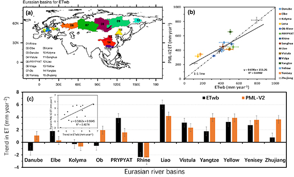
Figure 1. Validation of ET estimated by PML-V2 against observation-based ET derived by water-balance method. (a) Geographic locations of 15 river basins in Eurasia used for estimating basin-scale water-balance annual ETwb. (b) Comparing multi-year means and standard deviations of water-balance annual ETwb with those of annual ET from PML-V2 over 2003–2014. The coefficient of determination (R2) for each regression was calculated from all basin-to-year (∼180) ET data. (c) Summary of trends in annual ETwb and annual ET from PML-V2 for 12 Eurasian basins over 2003–2014.
Download figure:
Standard image High-resolution image2.4.2. Three types of long-term ET products
We compared PML-V2 estimates with other three types of ET products (GLEAMv3.3a, ERA5, and CRv1.0) which were estimated by entirely different methods. The GLEAM ET (version 3.3a) was estimated by the (GLEAM; available online https://www.gleam.eu/) that estimates global daily ET based on satellite-observed soil moisture, vegetation optical depth and snow-water equivalent, reanalysis air temperature and radiation, and a multi-source precipitation product (Martens et al
2017). In the GLEAM model, the cover-dependent potential evaporation ( ) is first calculated from the Priestley and Taylor equation, then
  is converted into
  or
or  using a vegetation cover-dependent, multiplicative stress factor S ranging from 0 to 1 (Martens et al
2017). The ERA5 ET was the output of the current reanalysis ERA5 of the European Centre for Medium-Range Weather Forecasts, available from 1979 to present (Dee et al
2011, Hersbach et al
2020). The CR ET was estimated by a calibration‐free nonlinear complementary relationship (CR) model (Szilagyi et al
2017, Ma and Szilagyi 2019) using input of surface climate forcing (air and dewpoint temperature, wind speed, and net radiation) that was mainly from the ERA5 reanalysis (Ma et al
2021). To our knowledge, the GLEAMv3.3a has partly included the impact of long-term change in vegetation cover, but the ERA5 and CR model do not consider this impact. Not like the PML-V2 model, all the three ET products do not consider CO2's impact on transpiration but provide a reference for PML-V2 ET estimates.
using a vegetation cover-dependent, multiplicative stress factor S ranging from 0 to 1 (Martens et al
2017). The ERA5 ET was the output of the current reanalysis ERA5 of the European Centre for Medium-Range Weather Forecasts, available from 1979 to present (Dee et al
2011, Hersbach et al
2020). The CR ET was estimated by a calibration‐free nonlinear complementary relationship (CR) model (Szilagyi et al
2017, Ma and Szilagyi 2019) using input of surface climate forcing (air and dewpoint temperature, wind speed, and net radiation) that was mainly from the ERA5 reanalysis (Ma et al
2021). To our knowledge, the GLEAMv3.3a has partly included the impact of long-term change in vegetation cover, but the ERA5 and CR model do not consider this impact. Not like the PML-V2 model, all the three ET products do not consider CO2's impact on transpiration but provide a reference for PML-V2 ET estimates.
3. Results
3.1. Validation of historical ET estimated by PML-V2
Firstly, we compared the historical annual ET estimated by PML-V2 with the observational annual ETwb derived over 2003–2014 from basin-scale water-balance method, and the result indicates a good performance of PML-V2 ET at basin scales (figure 1). Across 15 river basins in Eurasia, the PML-estimated annual ET are strongly correlated with the annual ETwb with a coefficient of determination (R2) of 0.70 (figure 1(b)). Due to different climate forcing used in the ET datasets, significant positive bias (∼11%) for all basins between the annual ETwb and the PML ET can be found (figure 1(b)), especially for the Yangtze River basin (∼30%) and the basins with small annual ET (e.g. the Kolyma, the Lena and the Yenisey rivers with biases of 50%–100%).
Secondly, we evaluated trends in annual ET over 2003–2014 (figure 1(c)). There are 12 out of 15 basins selected for trend analysis, since three basins (i.e. the Lena, the Songhua, and the Volga rivers) do not have complete annual streamflow data over 2003–2014. For the ETwb trends across the 12 basins, 8 out of the 12 have strong increasing trends, ranging from 0.8 to 6.0 mm year−2, while the basins with strong negative trends mainly locates at the Europe (e.g. the Danube and the Rhine rivers). In comparison, the PML-estimated ET in 10 out of the 12 basins have the same directions in trends of ETwb, with an R2 of 0.41 between trends in the two ET datasets (figure 1(c)). Relatively large differences (>50%) in trends between PML-V2 ET and ETwb can been seen for the basins of the Danube, Elbe, Ob, PRYPYAT, Yangtze and Zhujiang rivers (figure 1(c)). With area-weighted averaging applied over the 12 basins, the PML-V2 ET shows a trend of 1.83 mm year−2 over 2003–2014, which is close to the ETwb trend (1.57 mm year−2). These results indicate that the PML-estimated ET is adequate for further analysis of historical changes in ET and its driving factors' contributions over Eurasia.
3.2. Changes in environmental factors and ET over Eurasia during 1982–2014
With continually increased anthropogenic carbon emissions, global atmospheric CO2 has increased by 15.5% (∼56 ppm) over 1982–2014. In response to the CO2-induced climate change and vegetational fertilization, the annual LAI (or NDVI) over Eurasia has increased by 7.36% (or 5.79%) during this period (figure S2). The most significant increasing trends in LAI (>15%) or NDVI (>10%) can be found over the Europe, the Indian Peninsula and southeast China, occupying about 35% of the Eurasian area (figures 2(a), (b) and S3(a), (b)). The climate forcing over Eurasia has also experienced remarkable change (figures 2(c)–(f)), with surface air temperature (in °C) increased by 13.63%, and precipitation increased by 5.42% and other variables less than 5% (figure S2). The temperature increases exceed 20% over about 30% of the Eurasian land (figure S3(c)).

Figure 2. Long-term trends in vegetational and surface climatic variables over Eurasia during 1982–2014. (a), (b) Trends of annual NDVI and LAI derived from AVHRR GIMM3g datasets. (c)–(h) Trends of annual surface air temperature, precipitation, solar radiation, longwave radiation, specific humidity, and wind speed derived from the GLDASv2.0 dataset. The sub-histograms in (a)–(h) present land area fraction of trends at different levels corresponding to the color bars. The x-axis in each sub-histogram denotes a color map with the values of the same colors in the color bar.
Download figure:
Standard image High-resolution imageIn response to these increases in surface driving variables, the annual ET over Eurasia also has largely increased. By comparing the historical simulated ET trends from PML-V2 with the ERA5, GLEAMv.3.3a, and CRv1.0 ET products (figure 3), we find that all four ET datasets show significant increasing trends in ET over Eurasia for 1982–2014 (figure 3(a)). On area-weighted average over Eurasia, the GLEAM ET shows the largest trend (10.89 ± 0.90 mm year−1 decade−1, p < 0.01), followed by the PML ET trend (6.20 ± 1.13 mm year−1 decade−1, p < 0.01) and the CR ET trend (5.21 ± 1.15 mm year−1 decade−1, p < 0.01). The ERA5 ET trend is the smallest, but still strong (3.70 ± 1.05 mm year−1 decade−1, p < 0.01). It is worthy noted that uncertainty in trends between the four ET products may be due to different climate forcing used, but other important drivers (e.g. LAI, CO2) with large long-term trends whether being considered or not as input in the ET algorithms could strongly alter long-term change/trend of regional ET. In a word, the PML ET trend is close to the ensemble mean (6.51 ± 3.1 mm year−1 decade−1) of the other three. Spatial patterns of trends in ET are generally consistent within the four datasets (figures 3(c)–(f)). Most of high increasing trend values are from highly vegetated regions (about 60% of Eurasian area) over central and eastern Europe, the Indian Peninsula and southeast China where vegetation greening trends are largest (figures 2(a) and (b)). The ET trends over these high greening regions are larger than 20 mm year−1 decade−1 for both the PML-V2 and GLEAM datasets.

Figure 3. Comparison of long-term trends in annual ET over Eurasia during 1982–2014 from different products. (a) Timeseries of annual ET. (b) Boxplots for trends in ET. All trends are significant at a level of p < 0.01. (c) Spatial pattern for trend in annual ET estimated from PML-V2. (d)–(f) Same as (c) but obtained from GLEAMv3.3a, ERA5, CRv1.0, respectively. The sub-histograms in (c)–(f) present land area fraction of trends at different levels corresponding to the color bars. The x-axis in each sub-histogram denotes a color map with the values of the same colors in the color bar.
Download figure:
Standard image High-resolution image3.3. Contributions of dominant drivers to trend in ET over Eurasia
Using the historical estimations from PML-V2 driven by all observational forcings, we quantified the relative contributions of the three ET components, i.e.  ,
,  ,
,  to the long-term changes of annual ET during 1982–2014 over Eurasia (figures 4 and S4). On area-weighted average over the whole Eurasia, we estimated that the long-term increase in annual ET comes from the increases in
  and
and  , and the decrease in
  (figure 4(a)). The long-term trend in ET over Eurasia (6.20 mm year−1 decade−1) is primarily dominated by the increases in
  (4.18 mm year−1 decade−1) with a relative contribution of 61.1%. Although
  has a larger interannual variation over 1982–2014 than
  ,
,  has a much smaller contribution (−4.47%) to the trend of annual ET, while
  has a 34.46% of trend contribution (figure 4(b)). Regionally, the strong increase of ET over Eurasia is mainly from the highly vegetated regions where
  dominantly contributes 60%–80% of the ET trend (figures 4(c) and (d)). Over most of these regions,
  shows a negative contribution of 0%–20%, and
  contributes 0%–40% of reginal ET trends (figures 4(e) and (f)). For the desert or sparse vegetated regions such as the Arabian Peninsula, the Middle East, and the Qinghai–Tibet Plateau,
  dominates 80%–100% of the regional ET (positive or negative) trends (figures 4(c) and (e)).
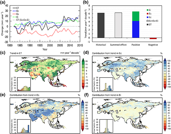
Figure 4. Contributions of ET three components (transpiration ( ), soil evaporation (
 ) and intercepted evaporation (
 )) to the long-term trend in ET over Eurasia during 1982–2014. (a) Timeseries of annual ET and its three components. (b) Boxplots for trends in ET and its three components. (c) Spatial pattern for trend in ET. (d) Spatial pattern for contributions of trend in
  to ET trend. (e), (f) Same as (d) but for
  and
and  , respectively. All data are derived from PML-V2 estimates for 1982–2014. Negative values in (d)–(f) indicate negative relative contributions (see equation (11)). The sub-histograms in (c)–(f) present land area fraction of trend contributions at different levels corresponding to the color bars. The x-axis in each sub-histogram denotes a color map with the values of the same colors in the color bar.
Download figure:
Standard image High-resolution imageWith the modeling sensitivity experiments using PML-V2 (see table 1), we further isolate the relative contributions of individual environmental drivers, i.e. climate forcing, CO2, LAI, albedo and emissivity, and their interactions (figures 5 and S5). We find that on area-weighted average, the summed effect of all individual drivers' contribution explains ∼87% of the trend in annual ET during 1982–2014 (figure 5). The nonlinear effect of driver interactions presents a negative contribution (∼13%) to the overall ET trend (figures 5(a) and (b)). Noticeably, we find that the timeseries of climate forcing-induced change in annual ET almost overlaps the historical change in annual ET driven by all drivers (figure 5(a)), indicating the dominant role of climate on both interannual variation and trend of ET over Eurasia. Due to the strong greening (an increase of 7.36% over Eurasia) over 1982–2014 as observed by satellites, the LAI alone has induced a strong increasing trend (3.88 mm year−1 decade−1) in annual ET. In contrast, the increased CO2 has resulted in a substantial decreasing trend (−4.67 mm year−1 decade−1) in annual ET (figures 5(a) and (b)), due to the CO2-induced suppression effect on  through reducing vegetational stomatal conductance (equation (4)). Consequently, the historical increasing trend in ET over Eurasia is mainly due to the positive relative contributions of changes in climate forcing (39.55%), LAI (21.94%) and surface albedo and emissivity (6.06%), and the negative relative contribution of increased CO2 (26.40%). Regionally, the dominance of climate forcing on ET trend covers 68.26% of Eurasian land area except for the South Asia and a part of western Europe where CO2 dominates (9.38%), and the India Peninsula and a part of northern Siberia where the LAI controls (13.06%, see figure 5(f)). Over most vegetation greening regions (figures 5(c)–(f)), such as central and eastern Europe and southeast China, the LAI-induced ET increasing trends (5–10 mm year−1 decade−1) are almost offset by CO2-induced ET decreasing trends (−10 to −5 mm year−1 decade−1). Even over the India Peninsula where LAI dominates the ET trends (15–20 mm year−1 decade−1), the CO2 has induced ET strong decreasing trends (−15 to −10 mm year−1 decade−1).

Figure 5. Contributions (%) of dominant drivers to the long-term trend in ET over Eurasia during 1982–2014. (a) Timeseries of annual ET induced by different environmental drivers. (b) Boxplots for trends in annual ET induced by different environmental drivers. (c)–(e) Spatial pattern for trends in annual ET induced by climate forcing, LAI and CO2, respectively. The sub-histograms in (c)–(e) present land area fraction of trends at different levels corresponding to the color bars. The x-axis in each sub-histogram denotes a color map with the values of the same colors in the color bar. (f) Spatial pattern for dominant driver of trends in annual ET. All data are derived from factorial simulations of PML-V2 (equations (7)–(10)). The pie chart in (f) presents the covered land area fraction of dominant drivers (albedo and emissivity, LAI, CO2, and climate), and unvegetated regions which are defined from the NASA MCD12Q1 IGBP land use and land cover types.
Download figure:
Standard image High-resolution image
4. Discussion
Most direct measurements of ET are primarily obtained from in situ observations based on the EC method (Baldocchi et al 2001, Wang and Dickinson 2012), but they are not able to be used for long-term change/trend analysis of ET or water cycle at large regional or global scales, e.g. over Eurasia in this study. This is due to the obvious shortages of the EC-based measurement that (a) the observed fluxes only represent local underlying surfaces and climatic variations which depends on the observation height, (b) current EC-based ET observations (e.g. the FLUXNET2015 dataset) still have limited spatial-to-temporal coverages. To estimate ET at regional or large scales using other observational information, many approaches have been proposed during past decades, such as EC data-driven machine-learning interpolation algorithms (Jung et al 2011, 2020), or remote sensing-based algorithms (Chen and Liu 2020), e.g. the Penman–Monteith equation (Mu et al 2007, 2011), the modified Penman–Monteith equation (Leuning et al 2008, Zhang et al 2015, 2019) and the Priestley–Taylor equation (Zhang et al 2010a, Martens et al 2017), or ground meteorological data-driven algorithms (Brutsaert 2015, Szilagyi et al 2017, Ma and Szilagyi 2019, Ma et al 2020, 2021).
The above remote sensing-based ET methods generally need parameter calibration using the EC-based ET and other variables measurements. In this study, the PML-V2, as a modified Penman–Monteith model, has been well-calibrated using the global 95 EC sites of the FLUXNET2015 dataset, and shows only slight degradation from the calibration to the cross-validation (figure S1). Compared to the independent observation-based ET derived from the basin-scale water balance method across 15 basins in Eurasia (figure 1), the PML-estimated ET also shows good performance (R2 = 0.70). Moreover, the PML-estimated ET agrees with the trend directions of water-balance based ET in 10 out of the 12 basins and is on area-weighted average close to the trend value of water-balance based ET, both indicating significant increase trends.
To estimate the long-term change in ET and its components (transpiration ( ), bare-soil evaporation (
 ), and rainfall interception loss (
 )), and to quantify the relative contributions of major drivers over Eurasia during 1982–2014, the parameter-calibrated PML-V2 model was applied to perform a group of modeling sensitivity experiments using observational climate variables, CO2, LAI, and albedo and emissivity as forcings. Consistent with previous studies (Zhang et al
2010a, 2016, Zeng et al
2014), the PML-based ET also suggested an increasing trend (6.20 ± 1.13 mm year−1 decade−1, p < 0.01) over Eurasia during 1982–2014 which is close to the ensemble mean (6.5 ± 3.10 mm year−1 decade−1) of the trends in other three ET products (GLEAMv3.3a, ERA5 and CRv1.0). The increasing trends were mostly from highly vegetated regions (about 60% of Eurasian area) over central and eastern Europe, the Indian Peninsula and southeast China where there were the strongest vegetation greenings.
)), and to quantify the relative contributions of major drivers over Eurasia during 1982–2014, the parameter-calibrated PML-V2 model was applied to perform a group of modeling sensitivity experiments using observational climate variables, CO2, LAI, and albedo and emissivity as forcings. Consistent with previous studies (Zhang et al
2010a, 2016, Zeng et al
2014), the PML-based ET also suggested an increasing trend (6.20 ± 1.13 mm year−1 decade−1, p < 0.01) over Eurasia during 1982–2014 which is close to the ensemble mean (6.5 ± 3.10 mm year−1 decade−1) of the trends in other three ET products (GLEAMv3.3a, ERA5 and CRv1.0). The increasing trends were mostly from highly vegetated regions (about 60% of Eurasian area) over central and eastern Europe, the Indian Peninsula and southeast China where there were the strongest vegetation greenings.
This study is clearly distinct from our previous PML studies for global ET patterns and trends. First, this study focuses on the relative contributions of ET's major external drivers to the long-term ET trends in Eurasia, especially for the relative importance of rising CO2 and increased LAI. This study, for the first time, find that the increasing ET trend induced by increased LAI over Eurasia can be largely offset by the rising CO2-induced reduction in stomatal conductance which strongly reduces transpiration. Second, this study used the latest version of PML-V2 model and the longest satellite-based LAI dataset (AVHRR GIMMS3g LAI) since 1980s. Our previous studies, however, focused on different scientific questions using an older version of PML model. For example, Zhang et al (2016) studied the global long-term trends of ET and estimated the earth greening (increased LAI's) contribution to the ET trends using the older version model—PML-V1 that does not consider the impact of rising CO2 on canopy stomatal conductance. Zhang et al (2017) still used PML-V1 to study on how climate drivers affect the spatiotemporal variation of soil respiration and transpiration. Zhang et al (2019) developed the latest version of PML model (PML-V2) that includes the rising CO2's impact on stomatal conductance and applied it to produce a coupled estimation of global ET and GPP at 500 m and 8 d resolution using the MODIS LAI since 2002. Zhang et al (2019) did not quantify the contribution of different external drivers (CO2, LAI, climate forcing, albedo etc) to the variations and trends in ET.
Previous studies have reported the strong contributions of historical increased LAI to the ET increasing trends at global and continental scales. For example, Zhang et al (2016) used the PML-V1 that did not consider CO2's impact on ecosystem water-use efficiency (or plant stomatal conductance) and indicated that the strong increased ET over Europe and Asia during 1982–2012 were dominated by enhanced  due to the increased LAI. Another study by Zhang et al (2015) used remote sensing-based ET to suggest the dominance of increased LAI and rising atmosphere moisture demand on long-term trends of global ET over 1982–2013. Using a coupled atmosphere-land global climate model (GCM), Zeng et al (2018) suggested that about 55% ± 25% of the observed global land ET increase during 1982–2011 was driven by the LAI increase. As the GCM also account for the impact of LAI on surface climate forcing, the large contribution of LAI on ET increase reported by Zeng et al included both direct contribution (i.e. LAI on
  ,
,  , and
, and  ) and indirect contribution (climate forcing on
  ,
,  , and
, and  ). In this study, we suggest that the increasing trend of ET over Eurasia was mainly contributed by climate forcing change (40%) and increased LAI (22%), but largely offset by increasing CO2-induced vegetational stomatal closure with a negative contribution of 26%. Due to the counteracting effect between the increased LAI and reduced vegetational stomatal conductance due to increased CO2, the resulted long-term change in ET over Eurasia was dominated by surface climate change and variability. This result implies that future estimations of global and regional ET considering only one impact from vegetational greening/growth or from the CO2's effect on stomatal closure (or ecosystem water-use efficiency) may induce systematical errors in the long-term changes in ET and the related water balance components.
5. Conclusions
Estimating ET trends and related causality analysis are great interest of hydrology and climate communities. Eurasia has experienced strong vegetation greening under increasing atmospheric CO2 concentration over the last four decades. It remains unclear how major ET drivers contribute to long-term ET changes and trends in Eurasia. This study uses a three-layer diagnostic water–carbon coupling model (PML-V2) to quantify relative contributions from four major ET drivers (LAI, climate forcing, atmospheric CO2, albedo and emissivity). The model performs similarly in detecting increased ET trends in Eurasia in 1982–2014, compared to other three global ET products. Furthermore, the PML-V2 ET trends compare reasonably well to the water balance-based ET trends in large river basins. Using PML-V2 for sensitivity analysis indicates that climate forcing change is a major contributor to the increasing ET trend in Eurasia (40%), while the positive contribution of LAI (22%) is largely offset by the negative contribution of CO2 (26%). Our results highlight the importance of counteracting effect between CO2-induced decrease in transpiration and LAI-induced increases transpiration and intercepted evaporation. This effect has not been considered by majority of remote sensing based diagnostic ET models, and hints that the long-term change of regional/global ET should be overestimated if the two opposite contributions are not considered together.
Acknowledgments
This work was supported by the CAS Pioneer Talents Program, the National Natural Science Foundation of China (42001019 and 41971032), and the Beijing Municipal Natural Science Foundation (8212017).
Data availability statement
The PML-V2 dataset in this study can be accessible from the corresponding authors upon request. The GLDAS version 2.0 climate forcing dataset is downloaded from https://ldas.gsfc.nasa.gov/. The GLASS albedo and emissivity datasets are obtained from www.glass.umd.edu/Download.html. The GLEAM ET dataset can be downloaded from www.gleam.eu/. The ERA5 ET dataset is available at www.ecmwf.int/en/forecasts/datasets/reanalysis-datasets/era5. The CR version 1.0 ET dataset is available at https://doi.org/10.6084/m9.figshare.13634552.v1.
The data that support the findings of this study are available upon reasonable request from the authors.