

Abstract
Emission inventory development for air pollutants, by compiling records from individual emission sources, takes many years and involves extensive multi-national effort. A complementary method to estimate air pollution emissions is in the use of satellite remote sensing. In this study, NO2 observations from the Ozone Monitoring Instrument are combined with re-analysis meteorology to estimate urban nitrogen oxide (NOX) emissions for 80 global cities between 2005 and 2019. The global average downward trend in satellite-derived urban NOX emissions was 3.1%–4.0% yr−1 between 2009 and 2018 while inventories show a 0%–2.2% yr−1 drop over the same timeframe. This difference is primarily driven by discrepancies between satellite-derived urban NOX emissions and inventories in Africa, China, India, Latin America, and the Middle East. In North America, Europe, Korea, Japan, and Australasia, NOX emissions dropped similarly as reported in the inventories. In Europe, Korea, and Japan only, the temporal trends match the inventories well, but the satellite estimate is consistently larger over time. While many of the discrepancies between satellite-based and inventory emissions estimates represent real differences, some of the discrepancies might be related to the assumptions made to compare the satellite-based estimates with inventory estimates, such as the spatial disaggregation of emissions inventories. Our work identifies that the three largest uncertainties in the satellite estimate are the tropospheric column measurements, wind speed and direction, and spatial definition of each city.
Export citation and abstract BibTeX RIS

Original content from this work may be used under the terms of the Creative Commons Attribution 4.0 license. Any further distribution of this work must maintain attribution to the author(s) and the title of the work, journal citation and DOI.
This article was updated on 2 March 2022 to improve the quality of the figures.
1. Introduction
Urban areas account for 55% of the global population and this number is expected to increase to 68% by 2050 (Ritchie and Roser 2018). In the future, city governments will have a larger fraction of air pollutant and greenhouse gas emissions under their purview, including nitrogen oxides (NOx = NO + NO2) and carbon dioxide (CO2). Evaluating the history of air pollutant emission trends in urban areas gives insight on the effectiveness of past and current urban policies to control these emissions, and gives a potential playbook for future policies.
Nitrogen dioxide (NO2) is a deleterious air pollutant primarily resulting from the high-temperature combustion of fossil fuels (Jacob 1999). It is linked to increased incidence of pediatric asthma (Gauderman et al 2005, Khreis et al 2017, Achakulwisut et al 2019), and respiratory-related mortality (Samoli 2006, He et al 2020). NO2, itself a noxious compound, also photochemically reacts in the atmosphere in the presence of volatile organic compounds to create ozone (O3) and fine particulate matter (PM2.5), additional harmful pollutants (Jacob 2000).
NO2 observations from satellite instruments have been informing the scientific community since the late 1990s (Burrows et al 1999, Leue et al 2001, Richter and Burrows 2002, Martin 2003). Utilizing observations from polar-orbiting satellite instruments can be especially powerful since a single instrument makes global measurements, as opposed to bottom up inventories that are built from a variety of reported datasets and vary in their rigor spatially. Satellite data are perhaps most often used in the quantification of long-term trends of NO2 concentrations (Duncan et al 2016, Krotkov et al 2016, Georgoulias et al 2019). Because of the short NO2 lifetime during the daytime (2–8 h), NOX emissions are highly correlated with NO2 column amounts (Stavrakou et al 2008, Kim et al 2009, Lamsal et al 2011, Duncan et al 2013). For this reason, satellite data have often been used to evaluate NOX emissions inventories.
Decreases throughout North America and Europe and recent emission reductions in China have been reported in widely used bottom-up inventories. In North America and Europe, satellite-based studies have shown that regional NOX emissions have dropped at a rate of approximately 3%–7% yr−1 since 2005 (Castellanos and Boersma 2012, Lu et al 2015, Zhang et al 2018, Silvern et al 2019, Goldberg et al 2019a, Macdonald et al 2021, Zara et al 2021) leading to 30%–70% reductions over a 15 year period. In China, there was a rapid NOX emissions increase in the 2000s (Richter et al 2005), peaking in 2012, and a subsequent decrease thereafter (Reuter et al 2014, De Foy et al 2016, Li et al 2018, Zheng et al 2018, Wang et al 2019). Elsewhere NOX emission trends have been mixed but generally have increased since 2005 (Lu and Streets 2012, Mahajan et al 2015, Duncan et al 2016, Geddes et al 2016, Barkley et al 2017, Georgoulias et al 2019, Itahashi et al 2019, Huneeus et al 2020, Hickman et al 2021, Vohra et al 2021). Going forward, Elguindi et al (2020) summarize that past scenarios that assumed strong pollution controls best represent the documented trends in the United States, Europe, and China, while low pollution control scenarios lie closest to actual trends in developing regions such as India and West Africa.
Top-down statistical methods to infer urban NOX emissions from satellite observations were originally developed using Ozone Monitoring Instrument (OMI) NO2 data in the 2005–2009 timeframe (Beirle et al 2011). Beirle et al (2011) quantified NOX emission rates from eight megacities. While satellite-based urban NOX emissions showed general agreement with city-reported inventories, Riyadh had a factor of three larger emissions rate than the reported inventory. The method utilized by Beirle et al (2011) has subsequently been validated and refined on known NOX emissions from power plants (De Foy et al 2015, Goldberg et al 2019b, Liu et al 2020). These studies find that the Beirle et al (2011) method performs best on the largest sources (uncertainties <30% for sources >10 Gg yr−1 NOX ), which have a consistent daily signal that is larger than the values ∼100 km upwind. Although the uncertainties can be fairly large for power plants, it is reasonable to think that the uncertainties for urban areas could actually be smaller because urban plumes are larger and more distinct from the upwind concentrations. An advantage of this technique over others (Canty et al 2015, Harkey et al 2015, Cooper et al 2017, Itahashi et al 2019, Visser et al 2019, Qu et al 2020) is that it does not rely on a chemical transport model, which are valuable tools, but involve an added layer of expertise and can be affected by model accuracy. Many prior studies quantifying NOX emissions using this top-down method apply it on a subset of megacities or power plants (generally fewer than ten) (De Foy et al 2015, Lu et al 2015, Lorente et al 2019, Goldberg et al 2019b, Liu et al 2020) due to computational expense, but here we exploit recent computational capabilities to apply the Beirle et al (2011) method to a larger set of urban areas (189 cities) during a longer timeframe (15 years). We also provide an evaluation in these regions against NOx emission estimates from multiple global bottom-up emission inventories.
2. Data and methods
2.1. OMI NO2
OMI is a passive spectrometer launched on the NASA Aura satellite in July 2004 and has been providing global observations of NO2 atmospheric column densities since 1 October 2004 (Levelt et al 2018). Aura is situated in a polar-orbiting flight path approximately 700 km above the Earth's surface with a Equatorial crossing time of 13:45 local time (Levelt et al 2006). Each day Aura has 14–15 orbits and was designed to have global coverage every day. Since the development of the 'row anomaly' in 2007 (Dobber et al 2008), which obstructs ∼30% of the field of view, it now has global coverage once every 2–3 days. OMI NO2 slant column densities are derived from backscattered radiance measurements in the 402–465 nm spectral window of the UV–Vis spectrometer (Marchenko et al 2015, Lamsal et al 2021). OMI measures backscatter radiances in a 2600 km swath with a nadir (center of the swath) pixel size of 13 × 24 km2. The consistency of the data record over a 16+ year period has allowed for numerous long-term evaluations of trace gas species (McLinden et al 2016, Levelt et al 2018, Liu et al 2018, Abad et al 2019, Shen et al 2019, Silvern et al 2019, Goldberg et al 2019a).
OMI NO2 data version 4.0 are operationally released by NASA (Lamsal et al 2021) (https://disc.gsfc.nasa.gov/datasets/OMNO2_003/summary). The version 4.0 update includes a high-resolution surface reflectivity product in the calculation of the air mass factor and a recently updated cloud scheme, but still has a low bias of approximately 50% in urban areas when compared to column observations from in situ measurements. We filter the Level 2 OMI tropospheric column NO2 data to ensure only valid pixels are used. Daily pixels with solar zenith angles ⩾80°, cloud radiance fractions ⩾0.5, and surface albedo ⩾0.3 are removed as well as the five largest pixels at the swath edges (i.e. pixel numbers 1–5 and 56–60). We also remove any pixel flagged by NASA including pixels with missing values and those affected by the row anomaly. The daily data are then re-gridded to a global 0.1° × 0.1° grid.
The uncertainty in any daily measurement in the operational data has been assigned to be approximately 1.0 × 10¹⁵ molecules cm−2 (Krotkov et al 2017). This equates to roughly a 5%–20% uncertainty over polluted areas. However, because we are oversampling over many days (>100 days), we assume that random errors will cancel due to the large number of observations used (Russell et al 2010). This leaves only the systematic errors, such as the air mass factor bias in urban areas, which we discuss in section 2.4.
2.2. OMI NOX emissions calculation
We use a top-down inverse statistical modeling technique to derive NOX emissions from a combination of satellite data and re-analysis meteorology. In this method, all OMI NO2 data over individual city centers or 'hotspots' are compiled and rotated based on the daily-observed wind direction, so that the oversampled plume is decaying in a single direction. We utilize the 100 m wind speed and direction from the ERA5 re-analysis dataset (Hersbach et al 2020) generated at 0.25° × 0.25°. For each city we use the closest gridded value without interpolation.
This top-down method can only be applied when NO2 is photochemically active and the NO2 lifetime is short. Wintertime has more erroneous data due to snow cover and the longer NO2 lifetime during wintertime yields urban plumes that are much more likely to overlap; both factors cause issues with the statistical fit. Therefore, we only use OMI NO2 data from May to September in the Northern Hemisphere north of 25° N, November–March in the Southern Hemisphere south of 25° S, and all monthly data in Equatorial regions between 25° N and 25° S. We do not expect any significant systematic biases due to this temporal filtering. We aggregate all daily satellite data into 3 year averages; 36 months of data for tropical regions and 15 months of data for extratropical regions. We choose 3 year averages in lieu of 1 year or a shorter timeframe in order to average out the noise in daily measurements and to account for the row anomaly which causes fewer available measurements in the later time record.
Once all daily plumes have been rotated to be aligned as an effective horizontal plume and averaged together during a three year period (usually 100–600 snapshots), we integrate ±0.5° along the y-axis about the x-axis to compute a one-dimensional line density in units of mass per distance. The line densities, which are parallel to the wind direction, peak near the primary NOX emissions source and gradually decay downwind as the NOX is transformed into different chemical species or deposited to the surface.
The line densities are fit to a statistical exponentially modified Gaussian (EMG) model (Beirle et al 2011, Valin et al 2013). This particular method was chosen due its ability to convert NO2 column information into NOX emission rates while accounting for meteorological influences and due to the multitude of studies verifying the methodology (De Foy et al 2014, Verstraeten et al 2018, Goldberg et al 2019c). A full description of the method can be found in the supplementary. An illustrative example of the method applied to Paris is shown in figure S1 (available online at stacks.iop.org/ERL/16/115004/mmedia). The five output parameters of the statistical fit are the: NO2 burden, NO2 background, decay distance, horizontal location of apparent source (ideally at the origin), and sigma of the Gaussian plume. The NOX emissions rate from the source can be calculated from the NO2 burden, decay distance, and NOX /NO2 ratio, which is assumed to be 1.33 (Beirle et al 2011, Valin et al 2011). In two final adjustments, the derived NOX emissions are multiplied by a factor of 1.37 (Goldberg et al 2019c) due to a known low bias in urban areas caused by coarse resolution a priori vertical profile information incorporated in the air mass factor, and then by a factor 0.77 to account for an early afternoon high bias in the emissions rate compared to the 24 h average emissions rate reported by annual inventories, using diurnal allocation factors described in Denier Van Der Gon et al (2011); sensitivity analyses of the early afternoon adjustment factor can be found in the supplementary. A discussion of the uncertainties associated with all multiplicative factors are noted in section 2.4 and the supplementary.
2.3. Bottom-up emissions estimates
We acquired gridded anthropogenic total NOX emissions data from five widely used inventories and projections (table 1): the Community Emissions Data System (CEDS) (McDuffie et al 2020), the Emissions Database for Global Atmospheric Research (EDGAR) version 5.0 (Crippa et al 2020), the Evaluating the Climate and Air Quality Impacts of Short-Lived Pollutants (ECLIPSE) version 5a (Klimont et al 2017), the Monitoring Atmospheric Composition and Climate CityZen (MACCity) project (Lamarque et al 2010), and the Shared Socioeconomic Pathways (SSP) projections (Riahi et al 2017). The two SSP scenarios displayed herein represent sustainability (SSP 1–1.9) and continued fossil fuel development (SSP 5–8.5) pathways.
Table 1. Summary of emissions inventories used for this study.
| Inventory | First year | End year | Resolution | Increment | Projection? |
|---|---|---|---|---|---|
| CEDS a | 1970 | 2017 | 0.5° × 0.5° | Annual | No |
| EDGAR v5.0 b | 1970 | 2015 | 0.1° × 0.1° | Annual | No |
| MACCity c | 1990 | 2020 | 0.5° × 0.5° | Annual | Yes, projection from 2000 |
| ECLIPSE v5a d | 1990 | 2050 | 0.5° × 0.5° | 5 year | 2020 only |
| SSP e | 2005 | 2100 | 0.5° × 0.5° | 5 year | Yes, projection from 2005 |
a https://zenodo.org/record/3754964 b https://edgar.jrc.ec.europa.eu/gallery?release=v50_AP&substance=NOx§or=TOTALS c https://eccad3.sedoo.fr/ d https://iiasa.acat/web/home/research/researchPrograms/air/ECLIPSEv5a.html e https://esgf-node.llnl.gov/search/input4mips/
The five inventories and their trends by region are shown in the supplementary (figures S2 and S3). In some cases, sectoral emissions needed to be added together to create total anthropogenic NOX emission files. The inventories report NOX emissions as 'equivalent' NO2, but the NO2/NOX ratio may vary by urban area, and can be considered a source of uncertainty. None of the inventories projected to 2020 include the effects of the COVID-19 lockdowns on air pollutant emissions.
All NOX inventories are re-gridded to a common spatial resolution of 0.05° × 0.05°, while retaining all original values at the coarser spatial resolution. A final emissions output file is created which lists the NOx emissions within radii of 0.1° to 0.75° at 0.05° increments of each city. We match the satellite-derived emissions to the emissions inventories using the sigma of the Gaussian plume which varies spatiotemporally. We assume that the satellite-derived emissions should be matched to a Gaussian radius of 2-sigma from the city center. The 2-sigma radius for all cities are provided in table S3. Varying the city radius between 1.5-sigma and 3-sigma will affect the magnitude comparison by ±30%, but has a lesser effect on the trend comparison (figure S4).
2.4. Methodological uncertainties
The total error associated with the magnitude of the top-down vs. bottom-up comparison is calculated to be 53%, and is the sum of the quadrature of seven potential sources of error: the tropospheric vertical column measurement in urban areas (30%), the wind speed and direction (25%), the collocation of the spatial extent between the top-down fit and bottom-up emission inventory (30%), the early afternoon to 24 h conversion emissions rate (10%), the 'clear-sky' bias (10%) which for these purposes is a result of emissions being different on clear-sky days compared to cloudy days, the NOx /NO2 ratio (10%) (Kimbrough et al 2017), and the random error of the statistical EMG fit (10%) (De Foy et al 2014). This total uncertainty is comparable to Verstraeten et al (2018), who quantified an uncertainty of 55% using this method with OMI NO2. For the trend analysis, the total uncertainty is much reduced, since the systematic uncertainties in the emissions are consistent throughout the time period, thus leaving only the random EMG fitting error of roughly 10% (De Foy et al 2014). For further information on this method or the uncertainties associated with this method, please see the discussion in the supplementary or other literature (De Foy et al 2014, Lu et al 2015, Verstraeten et al 2018, Goldberg et al 2019c).
3. Results and discussion
3.1. OMI NO2 trends
Regional NO2 temporal trends since 2005 have been well-documented (Duncan et al 2016, Krotkov et al 2016, Georgoulias et al 2019). We update the findings here to include the most recent years of annual data, and to narrow the focus on urban NOX emissions—instead of NO2 concentrations. We purposefully exclude 2020 data due to the emission anomalies associated with the COVID-19 lockdowns. In 2005, the global regions with the largest anthropogenic emissions were: eastern United States, western Europe, and east Asia. This is documented by both the 'top-down' OMI NO2 annual average of tropospheric vertical column NO2 and the 'bottom-up' CEDS inventory (figure 1; note the non-linear colorbars in each panel).

Figure 1. (a) OMI NO2 v4.0 annual 2005 tropospheric vertical column amounts. (b) Bottom-up annual 2005 NOX emissions from the CEDS inventory; units are Gg yr−1 NO2 per 0.5° × 0.5° grid cell; total in Tg yr−1 NO2 (c) OMI NO2 ratio between the 2012 and 2005 annual averages. (d) OMI NO2 ratio between the 2019 and 2012 annual averages. Areas with OMI NO2 annual values in either year smaller than 1015 molec cm−2 have been screened out in the bottom row panels.
Download figure:
Standard image High-resolution imageBetween 2005 and 2012, NO2 concentrations dropped dramatically (25%–40%) in North America, western Europe, and Japan in response to stringent policies enacted to reduce NOX emissions. Conversely, in China, India, and the Middle East, a lack of regional policies controlling NOX emissions yielded a further increase (+10%–50%) in the NO2 concentrations as compared to 2005 concentrations. Regional signals in Latin America, Africa, and Southeast Asia are mixed primarily due to the influence of biomass burning in these regions. In other locations, such as Central Asia, Northern Africa, and Oceania regional differences are dominated by natural variability due to sparse anthropogenic activities in these areas.
Between 2012 and 2019, NO2 concentrations either dropped or held steady in most global regions. The largest decreases during this timeframe were in eastern China. In very few regions, were there large obvious increases. NO2 changes between 2005 and 2019 at the regional level are displayed in figure S5.
3.2. OMI NOX emissions estimates for global megacities
Our top-down OMI NOX calculation converged for 80 (n = 80) global cities for the 15 year period of interest (2005–2019); 16 of them are shown in figure 2. We first performed the analysis on the 97 C40 cities (www.c40.org/cities), and found that the method generally does not work for metropolitan areas with population sizes of <2 million residents because of OMI's lack of sensitivity to their daily NO2 plumes. We then expanded our analysis to include all global urban areas with metropolitan area populations exceeding 2 million residents. In total, we performed the statistical fit on 189 global cities. In most cities (167 out of 189), the statistical fit converged in at least one out of the five 3 year periods of interest, but many cities did not have a full temporal range or the statistical fit would yield an unreasonably small effective NO2 lifetime (<0.5 h) and unusually large sigma (>100 km); these instances were excluded from our analysis because discontinuous estimates are harder to screen for reliability and trend consistency. Our method only works for cities isolated from other large cities within a 200 km radius. Examples of cities in which this method does not work due to insufficient isolation are Beijing, Shanghai, Kinshasa, Amsterdam, Boston, and Washington DC. The comparison between top-down OMI NOX emissions and the five bottom-up emissions inventories for all 80 cities can be found in figures S6−S15. We anticipated that C40 cities, a group of cities pursuing high ambition climate action, would have larger NOX reductions but we found no statistical difference between the trends in C40 cities and non-C40 cities since 2009 (figure S16).

Figure 2. OMI urban NOX emissions (black) for 16 global cities compared to six of the most widely used bottom-up NOX emissions inventories: CEDS (green), ECLIPSE/GAINS (light blue), MACCity (red), EDGAR (orange), SSP 1-1.9 (dark blue), and SSP 5-8.5 (violet). Note each city has a different y-axis. All 80 investigated cities are in figures S6–S15.
Download figure:
Standard image High-resolution imageWhen the 80 cities are grouped by region, patterns begin to emerge (figure 3). In the United States and Canada, top-down OMI NOX estimates were available for 14 cities (n = 14), and when combined together, matched the bottom-up inventories in both trend and magnitude to within ±10%; therefore, we assert no consistent bias in the urban NOX inventories for these two countries. Similarly, excellent agreement was generally found in Australia and New Zealand.

Figure 3. OMI urban NOX emissions for the 80 cities aggregated by global region.
Download figure:
Standard image High-resolution imageIn Europe (n = 13) and South Korea/Japan (n = 3), the temporal downward trends of NOX emissions match to within ±10%, but all the inventories appear to be underestimating the magnitude of NOX emissions. We have two hypotheses for this magnitude disagreement. This could be indicative of an error in the inventory caused by a large fraction of diesel vehicles in these countries, which are known to have been underestimated in the past (Anenberg et al 2017). Another hypothesis is that this could be indicative of daily lifestyle differences which would present itself in the mid-day to 24 h average conversion. For example, if the activities leading to NOX emissions in these countries are concentrated in the late morning or early afternoon, and less in the morning or evening due to a heavier reliance on public transit, then the mid-day to 24 h average multiplicative conversion factor should be lower. An additional hypothesis for Europe is that a longer NO2 lifetime due to Europe's extratropical latitudes is not being fully captured in our method.
In China (n = 6), we observe a broad peak in NOX emissions in the 2009–2012 timeframe, and subsequent reduction since 2012. Between 2012 and 2018, we calculate that urban NOX emissions decreased 35%, which was similar in magnitude to the urban NOX reduction between 2006 and 2012 in the United States and Canada (37%). When comparing to the satellite-based estimates, all bottom-up inventories appear to underestimate the rapid decrease in Chinese NOX emissions. The CEDS inventory, which uses the regionally-compiled MEIC inventory (Zheng et al 2018) with different spatial downscaling proxies, does capture the urban decreases, but not the extent—between 2012 and 2015, the gridded inventory reports a 7% decrease for the cities considered while the satellite data show a 22% decrease over the same 3 year period. On a national scale, reported Chinese NOX emissions decreased by 17% in the inventory between 2012 and 2015, but this larger decrease was driven by power plants located in rural locations. These findings are consistent with Zheng et al (2018) who also report that OMI NO2 downward trends are larger than the regional bottom-up inventory. They documented that downward trends in surface NO2 concentrations between 2012 and 2017 are smaller than the downward trends in the emissions inventory and satellite data; the ultimate reason for the disagreement is still unknown. However, the difference in this study is that we now account for the NO2 chemical lifetime, which has been documented to change over time and is responsible for some fraction of urban NO2 changes (Laughner and Cohen 2019).
In the Middle East (n = 11), all bottom-up inventories suggest a consistent increase in urban NOX emissions between 2006 and 2018, but the top-down OMI NOX estimates do not support this. Instead, the satellite measurements indicate that NOX emissions peaked in 2009, with a slow decrease in the following years. While urban NOX emissions still appear to be larger in 2018 than in 2006, the top-down estimate suggests only 10% larger as compared to 40%–60% larger as reported by the inventories. This discrepancy appears to be mostly driven by four cities (Dubai, Riyadh, Jeddah, and Karachi), which have shown relatively flat NOX emission changes between 2005 and 2018. In Latin America (n = 11) and Africa (n = 6), the narrative is similar to the Middle East in that projected upwards NOX emission trends in the later part of the time record (2012–2018) were in fact steady or downward trends. Scant country-level data exists on emissions or their trends for these regions to inform or validate the global inventories.
Top-down urban NOX emissions are most uncertain in India (n = 8). There are many reasons for this. First, the satellite measurements in India, especially Delhi, are most affected by aerosol interference as compared to other urban areas around the globe (Vohra et al 2021). Because of this bias, top-down urban NOX emissions are likely biased low in this region. Satellite measurements in India are also biased by the wet monsoon (limited measurements) and dry monsoon (long-range transport from biomass burning may influence the urban calculation). Further, Indian bottom-up inventories sometimes show unrealistic changes, such as the 31% drop in the EDGAR-reported Delhi NOX emissions between 2011 and 2012. Sharp changes in the inventory at the urban scale are likely due to the downscaling/disaggregation of national emissions because national trends do not have similar sharp changes (figure S3). With that said, urban area NO2 trends are noticeably different when compared to the relatively rural, but highly industrial areas of east central India (Chhattisgarh and Jharkhand). In the largest Indian cities (e.g. Delhi, Mumbai, and Kolkata), NO2 trends are relatively flat between 2005 and 2019, while there have been large increases in east central India (figure S5). This may suggest an issue in the spatial disaggregation of emissions as opposed to an error in the national inventory.
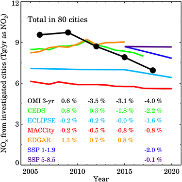
When summing all urban areas in our study, (n = 80), we find that satellite-based measurements show a larger decrease in global urban NOX emissions than currently reported in the inventories or projections (figure 4). Between 2009 and 2018, the satellite measurements indicate that urban NOX emissions dropped by 3%–4% yr−1, while the inventories and projections suggest drops generally less than 2% yr−1. The OMI observed NOX reductions in the 2015–2018 timeframe are most similar to the CEDS inventory (2.2% yr−1) and the SSP 1–1.9 projection (2.0% yr−1) as seen in figure 4. The CEDS inventory captures the recent global decreases best, presumably because it relies more heavily on country-inventory data. ECLIPSE (a projection between 2015 and 2020) and MACCity (a projection throughout the entire timeframe) both show a steady decrease over time (∼1% yr−1), but fail to capture the dramatic drops starting 2012. The EDGAR inventory likewise does not capture the drop starting in 2012. We attribute this to an underestimation of Chinese decreases as well as slower increases in developing nations such as Latin America and Africa (Hickman et al 2021) in the 2012–2018 timeframe.
Figure 4. OMI urban NOX emissions for the 80 cities aggregated globally. The % change per year at four time intervals (2009, 2012, 2015, 2018) where applicable are also shown for the satellite-based estimates and six inventories.
Download figure:
Standard image High-resolution image
4. Conclusions
In this study, we calculate anthropogenic urban NOX emissions and their trends in 80 global megacities during 2005–2019. Generally, top-down and bottom-up urban NOX emission trends show good agreement in North America, Europe, Korea/Japan, and Australasia. In China, bottom-up inventories fail to capture the timing of urban emission reductions, which appear to have occurred faster in the 2012–2015 timeframe than currently reported. In developing nations (Latin America, Africa, India) it appears that large projected increases in NOX emissions have not materialized to date. As a result, satellite-based measurements, when aggregated globally, show a larger decrease in urban NOX emissions than currently reported in the inventories in the 2009–2018 timeframe.
It should be noted that global inventories have to make assumptions about the spatial distribution of sources, such as power plants and vehicles. For example, power plants near urban areas may be more likely to be subject to greater emission controls than those located elsewhere in a country. In addition, passenger and freight vehicles likely have different spatial and temporal distributions. These types of distinctions are less likely to be captured in global gridded datasets, compared to region-specific inventories such as the U.S. National Emissions Inventory. Therefore, a portion of the disagreement may not be due to errors in the national-level inventory, but instead a misallocation of the spatial (and implied temporal) distribution (e.g. Huneeus et al 2020). Therefore, the NOx emission trends reported here are specific to the cities studied and are not necessarily reflective of national trends.
The distinct advantage of our methodology is the ability to isolate urban emissions at the global scale, while accounting for lifetime differences driven by meteorology and chemical nonlinearities. Further our method directly accounts for meteorological (Goldberg et al 2020) and chemical lifetime (Laughner and Cohen 2019) differences between regions which are important and can be difficult to disentangle. For example a city in an Equatorial region (e.g. Singapore) will have smaller NO2 concentrations due to the smaller solar zenith angle and faster photolysis than an extratropical city (e.g. Paris) with equivalent NOX emissions. Similarly, NO2 columns can be up to three times smaller on days with winds >8 m s−1 as compared to days with winds <2 m s−1 given equivalent NOX emissions (Goldberg et al 2020).
However, it should be noted that there is a cross-dependence of fitted effective NO2 lifetime and satellite-derived NOX emissions. The derived NOX emissions reported herein will increase with a shorter effective NO2 lifetime and decrease with a longer effective NO2 lifetime, under a scenario of constant NO2. The parameters that are used to calculate the NO2 lifetime are the wind speed and exponential decay length scale, which means that this method is particularly sensitive to wind speed, wind direction, and the sources downwind of an urban area; the latter two variables affect the fitted exponential decay length scale. A consistent low bias in wind speed, for example, would decrease the effective NO2 lifetime, and increase the derived NOX emissions. A consistent source downwind of an urban area, such as a smaller city, would increase the effective NO2 lifetime, and decrease the derived NOX emissions. Effective NO2 lifetimes for all cities are provided in table S4.
Future work to reduce the methodological uncertainties should focus on comprehensively testing this method using a global chemical transport model at high spatial resolution. While this has been done previously using a regional model for Atlanta (De Foy et al 2014), differences in local conditions can be substantial sources of error and are hard to account for. For example, the air mass factor and local meteorology can vary substantially between cities, and while some effort was made to account for these differences, our assumptions were broad and sometimes used coarse spatial resolution datasets. Better quantifying errors in the winds/plume speed and vertical distribution of NO2 through in situ observations or even satellite data itself (Liu et al 2021) at various times of the days will also be crucial to reducing the uncertainty. Long-term records from remote sensing instruments with higher spatial resolution and higher signal-to-noise ratios, such as the Tropospheric Monitoring Instrument (Veefkind et al 2012), Tropospheric Emissions: Monitoring Pollution (Zoogman et al 2017), Geostationary Environment Monitoring Spectrometer (Choi 2018), will further reduce the uncertainties in our top-down emissions method and provide estimates at higher temporal (daily/monthly) resolution (Griffin et al 2019, Lorente et al 2019, Goldberg et al 2019b, 2021). Future applications of this technique may be valuable for urban policymakers who want to better quantify changes in their air quality footprint over decadal timeframes, and track progress towards policy goals. Satellite datasets, as a stand-alone product, should not be used to determine compliance, but instead could be used as one of many metrics to assess progress.
Acknowledgments
This publication was developed using funding from the NASA Atmospheric Composition Modeling and Analysis Program (ACMAP) (80NSSC19K0946), NASA Health and Air Quality (HAQ) program (80NSSC19K0193), and NASA Health and Air Quality Applied Sciences Team (HAQAST) (80NSSC21K0511). This publication was also partially funded by the Department of Energy, Office of Fossil Energy and Carbon Management. OMI NO2 data can be freely downloaded from the NASA website (doi: 10.5067/Aura/OMI/DATA2017). ERA5 re-analysis hourly data on single levels can be downloaded from Copernicus Climate Change Service (doi: 10.24381/cds.adbb2d47).
Data availability statement
The data that support the findings of this study are openly available at the following URL/DOI: https://doi.org/10.6084/m9.figshare.14807565. Data will be available from 18 October 2021.