

Abstract
Tropospheric NO2 columns retrieved from ozone monitoring instrument (OMI) are widely used, even though there is a significant loss of spatial coverage due to multiple factors. This work introduces a framework for reconstructing gaps in the OMI NO2 data over China by using machine learning and an adaptive weighted temporal fitting method with NO2 measurements from Global Ozone Monitoring Experiment–2B, and surface measurements. The reconstructed NO2 has four important characteristics. First, there is improved spatial and temporal coherence on a day-to-day basis, allowing new scientific findings to be made. Second, the amount of data doubled, with 40% more data available. Third, the results are reliable overall, with a good agreement with Multi-AXis Differential Optical Absorption Spectroscopy measurements (R: 0.75–0.85). Finally, the mean of reconstructed NO2 vertical columns during 2015 and 2018 is consistent with the original data in the spatial distribution, while the standard deviation decreases in most places over Mainland China. This novel finding is expected to contribute to both air quality and climate studies.
Export citation and abstract BibTeX RIS

Original content from this work may be used under the terms of the Creative Commons Attribution 4.0 license. Any further distribution of this work must maintain attribution to the author(s) and the title of the work, journal citation and DOI.
1. Introduction
Nitrogen dioxide (NO2) is an important trace gas with a short atmospheric lifetime that has impacts on troposphere ozone (Tiwari and Agrawal 2018, Kang et al 2020) and secondary nitrate aerosols (Wang et al 2011a). Nitrogen oxides (NOx ≡ NO + NO2) are produced through atmospheric combustion associated with the recent industrialization process in China, with many cities still suffering from harmful air pollution (Richter et al 2005, Cohen and Prinn 2011, Zhang et al 2012a, 2012b, Zhao et al 2013), although there has been a recent decrease in some parts of China over the past few years (Gu et al 2013, de Foy et al 2016, van der A et al 2017, Si et al 2019, Wang et al 2019, Georgoulias et al 2019). Furthermore, since NO2 is known to have adverse impacts on human health and ecosystems (Atkinson et al 2018), it should be monitored dynamically and regularly on a large scale.
Satellite retrieval of NO2 offers a tool for monitoring the spatial distribution and temporal variation of tropospheric NO2 (Bovensmann et al 1999, Burrows et al 1999, Levelt et al 2006, Veefkind et al 2012, Yang et al 2014, Munro et al 2016, Kim et al 2020, Liu et al 2020b). Specifically, the ozone monitoring instrument (OMI) is the first sensor to provide daily global coverage of NO2 at a relatively high resolution (Levelt et al 2018), becoming widely used in air quality applications, including estimation of ground-level NO2 concentrations (Lamsal et al 2008, Lee and Koutrakis 2014, Qin et al 2017, 2020, Zhan et al 2018, de Hoogh et al 2019), spatiotemporal analysis of tropospheric NO2 columns (Cui et al 2019, Si et al 2019, Wang et al 2019), calculation of top-down NOx emissions (Liu et al 2016, 2017a, Silvern et al 2019, Kong et al 2019, Adams et al 2019), assimilation of observations into chemical transport models (Wang et al 2011b, 2020, Silver et al 2013, Liu et al 2017b). However, the OMI dataset tends to be used for long-term (monthly, seasonal or annual) analysis because of a row anomaly issue, which sacrifices the temporal resolution and contributes to an artificially high standard deviation (Cohen 2014, Cohen et al 2018, Lin et al 2020). Another significant issue is the cloud contamination, which can bias the results by obscuring the sensor's view of the lower atmosphere, resulting in significant errors, particularly in polluted regions (Boersma et al 2004).
Geostatistical methods such as inverse distance weighting and kriging interpolation are conventionally applied to predict values using neighboring information. They may lead to spatial discontinuity if the gap is large, while also not taking the temporal relationship into account, making the reconstruction of atmospheric products complicated (Shen et al 2015). Peng et al (2016) extend the adaptive weighted temporal fitting (AWTF) method to reconstruct OMI total ozone columns. However, the lack of information caused by clouds makes it impossible for tropospheric NO2 data products to meet the premise of AWTF (where 90% of the target data gaps have an overlap with valid values occurring either the previous or next day). de Hoogh et al (2019) impute missing OMI NO2 columns over Switzerland using estimates from a chemical transport model, with a linear regression model explaining 68% of the variability, demonstrating the feasibility of using another NO2 product to fill the gaps associated with OMI (which has an afternoon overpass), such as the Global Ozone Monitoring Experiment–2B (GOME-2B) (which has a morning overpass).
The relationship between tropospheric NO2 loadings in the morning and the afternoon changes under different land use and meteorological conditions (Lin et al 2010, Wang et al 2017a, Weng et al 2020, Penn and Holloway 2020) and due to its complexity, ordinary linear regression cannot fit it well (Cohen and Prinn 2011). Thus, we first use a machine learning method to capture the nonlinear relationship, and second apply AWTF to further improve the data coverage. This research aims to combine GOME-2B NO2 column data with OMI NO2 data to overcome these known issues and use the additional benefit of a different overpass time, with the goal of producing a more robust, precise, and scientifically useful NO2 dataset over China.
2. Data and methods
2.1. Data used in the model
OMI onboard Aura (2004–today) has a local equator crossing time at around 13:45 providing early afternoon coverage globally. OMI measures backscattered solar UV, allowing the approximation of the NO2 vertical column with an overall spatial resolution of 13 km × 24 km at nadir (Levelt et al 2006, 2018). This work uses the QA4ECV NO2 version 1.1 provided by KNMI (Boersma et al 2017), which features an enhanced spectral fitting method (Zara et al 2018) and improved air mass factor calculation (Lorente et al 2017, 2018) and shows a good agreement with ground-based measurements (Boersma et al 2018, Liu et al 2019) over China with a 12% total uncertainty at Xianghe (Compernolle et al 2020).
Several criteria are used to ensure the data quality according to the standard L3 product production process (Krotkov et al 2017), including: first, setting the cloud fraction <0.3, second, setting the surface albedo <0.3, and third, setting the solar zenith angle <85°. To further ensure quality, cross-track pixels affected by row anomalies are excluded. This row anomaly was first noticed in June 2007, and since 2009 has affected around one-third of the cross-track positions (http://projects.knmi.nl/omi/research/product/rowanomaly-background.php#overview).
GOME-2 on MetOp-B (2012–today) is a nadir-scanning spectrometer, which measures at around 9:30 local equator crossing time. The default ground pixel size of GOME-2B is 80 km × 40 km in the forward scan, requiring 1.5 d to cover the globe (Munro et al 2016). The GDP offline products of version 4.7 and 4.8 provided by DLR in the framework of the EUMETSAT AC-SAF project are used here. To be compatible with each other, all OMI and GOME-2B NO2 tropospheric columns were binned to 0.25° × 0.25° grids using HARP, a toolkit for binning weighted polygon-shaped remotely sensed measurements, as given by (http://stcorp.github.io/harp/doc/html/index.html).
To ensure that data from two satellites are available, all products in this work are subsequently confined to the same study period, specifically from 1 January 2015 to 31 December 2018, with specific details summarized in table S1.
Hourly concentrations of ground-level NO2 from 2015 to 2018 from the China National Environmental Monitoring Center (CNEMC) website were averaged during both the morning (0900 and 1000 Local solar time, LST = UTC + 8) and the afternoon (1300 and 1400 LST). The ordinary kriging method (Núñez-Alonso et al 2019) was used with month-by-month NO2 data to produce spatially continuous ground-based NO2 concentration maps.
Given that the air quality is closely related to meteorological conditions (Guo et al 2017, 2019), five instantaneous meteorological variables, including 10 m U and V wind components (u10 and v10; unit: m s−1), the 2 m air temperature (t2m; unit: K), boundary layer height (blh; unit: m), and surface pressure (sp; unit: hPa), at a 0.25° × 0.25° resolution were downloaded from the ERA5 hourly atmospheric reanalysis. Daily meteorological variables were averaged from 1100 to 1300 LST data, so as to coincide with the overpass time of two satellites.
Land cover types are considered to distinguish different types and magnitudes of anthropogenic activity in different places. The specific product contains nine land types (Cropland, Forest, Grassland, Shrubland, Wetland, Water, Tundra, Impervious Surface, Bareland) from the Finer Resolution Observation and Monitoring of Global Land Cover (FROM-GLC) 2017v1 dataset (Gong et al 2013), with a spatial resolution of 30 meters. The two types (impervious surface and cropland) were used for building the model, and the spatial scale was fractionally aggregated type-by-type to a spatial resolution of 0.25° × 0.25°.
2.2. Other data used in this work
The TROPOspheric Monitoring Instrument (TROPOMI) on Sentinel-5 Precursor (2017–today) has a significant raise in spatial resolution (3.5 km × 7 km initially, and 3.5 km × 5.5 km from August 6 2019 onward) and a similar equator crossing time of 13:30 with OMI (Veefkind et al 2012). The offline or reprocessing products of version 1.2.0 and 1.2.2 from 1 May 2018 to 31 December 2018 are used to make a comparison with our reconstructed data, and pixels with qa_value <0.75 are filtered to ensure the data quality.
We also used Multi-AXis Differential Optical Absorption Spectroscopy (MAX-DOAS) measurements at two suburban sites (see locations in figure S1 (available online at stacks.iop.org/ERL/15/125011/mmedia)) to evaluate the performance of reconstructed data, including one in Xianghe (116.96º E, 39.75º N) to the south of Beijing, and another at the roof of the School of Environment Science and Spatial Informatics in Xuzhou (117.14º E, 34.22º N). The instrument in Xianghe was designed at BIRA-IASB (Clémer et al 2010) and the data before January 2017 can be downloaded from http://uv–vis.aeronomie.be/groundbased/QA4ECV_MAXDOAS/index.php. The instrument in Xuzhou is a MAX-DOAS 2000 which was developed by the Anhui Institute of Optics and Fine Mechanics (Wang et al 2017b), and data are available from March 2018. We averaged all valid MAX-DOAS measurements within ±1 h of the OMI overpass time for comparison with the satellite data of the single grid cell where the site is located.
2.3. Reconstruction framework
The framework used to systematically create the reconstructed NO2 product (see figure 1) is based on two steps. First, the OMI and GOME-2B data are combined using The eXtreme Gradient Boosting (XGBoost) approach, a gradient boosting tree machine learning algorithm (Chen and Guestrin 2016), to form the first reconstruction step (RECON-1). This step regresses by producing a prediction model in the form of an ensemble of weak predictions (Chen and Guestrin 2016, Mitchell and Frank 2017), which has been shown to be applicable in various remote sensing applications (Hengl et al 2017, Just et al 2018, Shtein et al 2019, Li et al 2020). Specifically, this approach combines information that exists in GOME-2B to provide information that was otherwise missed by the same OMI pass later that same day.
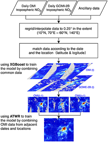
Figure 1. The flowchart of the reconstruction framework.
Download figure:
Standard image High-resolution imageThe second systematic step to create the reconstructed NO2 product requires filling missing data using the AWTF method (Peng et al 2016). This makes use of the information at the target location the day before and the day after (t− 1 and t + 1) to predict the target at date t (RECON-2). Specifically, the regression relationship is calculated from the grid cells in the adaptive search window with valid values over the three-day window, effectively considering the spatial-temporal patterns of NO2. The AWTF method computes RECON-2 with respect to the subset of grid cells, which have neither OMI nor GOME-2B valid data, thus further improving the spatial coverage.
NO2 data from OMI and GOME-2B, as well as ancillary surface and meteorological data in table S1 are interpolated onto a common grid in space and time. XGBoost is first applied to combine common data, and the relationship is trained by using the features (all listed in table S1 except omi) to predict a target variable (omi). ATWR is subsequently applied to predict missing data using adjacent measurements in space and/or time of RECON-1. The principles of XGBoost and AWTF are summarized in text S1 and text S2.
Before applying the XGBoost tree-based models, in this work the OMI NO2 column loadings are scaled using a natural log-transformation (figure S2). Using the log-transformed data, a tenfold cross validation to tune the hyperparameters for training the model was conducted to avoid errors due to random sampling. The 6 668 046 matching grid cells from 2015 to 2018 were divided each turn into a training set (90%) and a validation set (10%). The results of the model performance are analyzed using three metrics: the root mean square error (RMSE), the mean average error (MAE), and the coefficient of determination (R2) (equations (1–3)),
where  and
and  denote the model predicted vertical column and the OMI measured vertical column respectively,
  denotes the mean of
  and
and  denotes the number of samples.
Resulting scatterplots of the training and testing splits from 2015 to 2018 over mainland China are given in figure 2. Overall, the model performs well with MAE = 0.66 × 10¹⁵ molecules cm−2, RMSE = 1.54 × 10¹⁵ molecules cm−2, and R2 = 0.89. However, there is a small underestimation of the NO2 vertical column at high values (greater than 80 × 1015 molecules cm−2).

Figure 2. Scatterplots of model fitting cross-validation results of all daily vertical column density measurements (x-axis) and predictions (y-axis) over Mainland China. The black and orange lines represent the 1:1 and best-fit linear regression lines, respectively.
Download figure:
Standard image High-resolution image3. Results and discussions
3.1. Day-by-day reconstruction and analysis
The reconstructed data show improvement over OMI and either improvement over or similarity to the higher spatial resolution TROPOMI in terms of spatial coverage. First, there is a significant improvement over regions with missing data, due to either the known OMI row anomaly (red color) or extensive cloud cover (blue color), as clearly demonstrated in a specific case from 31 October to 2 November 2018 (figure 3, RECON-1). Second, there is a further reduction of missing data due to the inclusion of information over the three consecutive day period during which at least one input dataset has valid data (such as the grey dashed grid boxes) (figure 3, RECON-2).

Figure 3. 31 October, 1 November, and 2 November 2018 OMI tropospheric NO2 vertical columns generated by the reconstruction framework and measured by TROPOMI. The three columns represent the three dates respectively, with the first row (a–c) showing the original OMI measurements, the second row (d–f) showing RECON-1, the third row (g–i) showing RECON-2, and the final row (j–l) showing the measured TROPOMI NO2 vertical columns. The red grid boxes represent the data missing due to OMI row anomaly, while the blue due to cloud cover. The grid boxes with solid lines are reconstructed in the first step, while those with dashed lines in the second step. The grey dashed box is just a reference for showing the same area over the consecutive days.
Download figure:
Standard image High-resolution imageThe tropospheric NO2 vertical columns in the reconstructed data are consistent with the various measurements that exist within the area of overlap, without showing distinct boundaries. RECON-2 and TROPOMI both identify most of the hot spots of tropospheric NO2, with the following caveats. Although the spatial resolution of TROPOMI is superior to OMI where both products exist, there are also regions over which TROPOMI has no data (due to cloud contamination or lower data quality), but the reconstructed OMI NO2 product does have data, such as hotspots in the Pearl River Delta, Henan, and Xinjiang, and the lesser polluted regions in Yunnan and Inner Mongolia. One result is that RECON-2 tropospheric NO2 columns are on an average higher than TROPOMI (16.0%), consistent with the fact that such measurements overall tend to underestimate actual NO2 (Verhoelst et al 2020) and the fact that RECON-2 tends to have a lower fraction of missing data over highly polluted regions, as compared to TROPOMI.
An important insight is made by exploring and analyzing the reconstructed NO2 data from 15 March 2017 (figure 4). This date was selected because there is a total absence of OMI data from the 14 to the 16 due to acquisition problems, which would normally render any scientific analysis impossible on these days. However, the reconstructed result provides a significant amount of data for analysis, allowing for a scientific result to be achieved on the 15, where previously no possibility existed. First of all, the known spatial distribution of high NO2 column loading over the Beijing-Tianjin-Hebei region is still present, but it is shown to also extend into the northern and western parts of Shandong as well as through the western and southern part of Jiangsu. Secondly, over this region as a whole (except for Beijing itself) the difference between RECON-2 and GOME-2B shows a reduction on average, which is in fact completely consistent with the extremely high temperatures observed during this time (figure 4(e)). Thirdly, the elevated NO2 vertical column loadings over Henan, Shanxi, Shaanxi, and Hubei is not normally observed, but is found to be completely consistent with the strong winds and subsequent long-range transport observed during this time (figure 4(d)). This indicates that there is not only a practical increase in data coverage using this technique but also an increase in the ability to make important scientific discoveries, frequently which have important scientific differences under difficult conditions of very cloudy or heavily polluted (and usually treated as clouds by remotely sensed measurements).
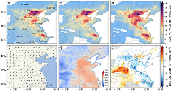
Figure 4. The spatial distribution of the tropospheric NO2 vertical column over Central Eastern China on March 15 2017 from: (a) RECON-2, (b) RECON-1, (c) GOME-2B, and (f) the difference between RECON-2 and GOME-2B. ERA5 wind and temperature conditions during the satellite overpass times are shown in (d–e), respectively.
Download figure:
Standard image High-resolution image3.2. Climatological analysis
The spatial distribution of the OMI data coverage (the ratio of the number of days that each grid cell has valid data to the total 1461 d) from 2015 to 2018 is compared in figures 5(a)–(c), and the amount of reconstructed data is twice as much as that of the original data. Overall, the data coverage is improved by more than 40%, with the percentage of grid cells where OMI has no value in mainland China dropping from 63% to 22% in general.
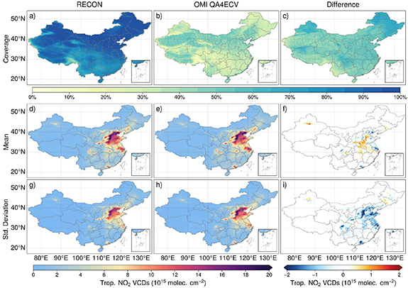
Figure 5. Statistics of daily tropospheric NO2 VCDs from 2015 to 2018: (a) reconstructed coverage, (b) OMI coverage, (c) difference between reconstructed coverage and OMI coverage, (d) reconstructed mean, (e) OMI mean, (f) difference between reconstructed mean and OMI mean, (g) reconstructed standard deviation, (h) OMI standard deviation, (i) difference between reconstructed standard deviation and OMI standard deviation.
Download figure:
Standard image High-resolution imageThe statistics of the mean NO2 vertical columns during 2015 and 2018 from the reconstructed results and original measurements show a significant amount of similarity overall, including a high level of consistency in terms of the spatial distribution, as demonstrated in figures 5 (d)–(f). It should be noted that some of the most polluted regions (the Beijing-Tianjin-Hebei region, the Yangtze River Delta region, the Pearl River Delta region, and Chengdu) show a moderately lower mean (about −2.3%), while some of the regions (Henan, Hubei, Hunan, Jiangxi, Anhui, Liaoning, Jilin, and Heilongjiang provinces) show a slightly higher mean (about +1.1%). Due to the inclusion of the filling of missing data, the drop in the standard deviation of the reconstructed OMI NO2 VCDs has been shown over almost all of China (roughly −10.4%), as shown in figures 5(g)–(i). The only two minor exceptions are both found in small portions of rapidly developing energy regions in Northern Xinjiang and Jilin (+16.2%), and the reconstructed result has a larger mean (up to +12.9%) at the same time, which is possibly due to a rapidly changing emissions source and access to a greater amount of underlying data (Lin et al 2020).
3.3. Data evaluation
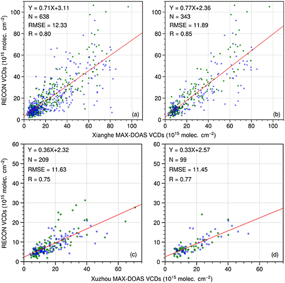
A comparison is made between the reconstructed NO2 columns and measurements from MAX-DOAS as shown in figure 6. Following previous work (Lin et al 2014, Liu et al 2019, 2020a) a filter is applied to remove all MAX-DOAS data whose standard deviation exceeds 20% of their mean value, as a method to exclude local pollution events near the MAX-DOAS site. The results both without filter (figure 6(a), (c)) and with filter (figure 6(b), (d)) are provided. When the OMI QAECV data has a valid value, the reconstruction result still uses the original value, so match-up points are separated using blue and green colors, which represent the original OMI value and the newly added data relative to QA4ECV, separately. A good agreement of the Pearson correlation coefficient (R) between 0.75 and 0.85 is found between them in the two sites.
Figure 6. Scatter plots for tropospheric NO2 VCDs between the RECONstructed data and MAX-DOAS in Xianghe (a–b) and Xuzhou (c–d). MAX-DOAS data are not filtered in the first column, while they are filtered in the second. The green dots represent the data from OMI QA4ECV product itself and the blue dots represent the newly added data relative to QA4ECV.
Download figure:
Standard image High-resolution image
The filtered comparison between them has a better R and a lower RMSE, while the number of match-up points drops by a half. The detailed results of each item are listed in tables S2–S5. It seems that the reconstructed product has a slightly inferior performance. After calculating the mean value and standard deviation of the MAX-DOAS in the corresponding dates, no matter whether the filter is applied or not, the NO2 columns from MAX-DOAS have a higher NO2 loading when comparing to the reconstructed NO2 columns, as compared to the OMI QA4ECV only. There is a bias in the satellite NO2, which possibly comes from both the retrievals and the emissions. In reality, the inclusion of more data points has allowed us to both simulate the higher values of the NO2 column loadings (consistent with the measured conditions) as well as to reduce the variance around these higher values. It should be noted that some regional data products partly correct the retrieval bias via improving air mass factor, such as POMINO (Lin et al 2014, 2015, Liu et al 2019) over China, HKOMI (Kuhlmann et al 2015) and BEHR-HK (Mak et al 2018) over the Pearl River Delta region, which deserve further study and comparison.
The time-series changes of daily tropospheric NO2 columns derived from the reconstructed product and MAX-DOAS without a filter are shown in figures S3–S4, demonstrating that the reconstructed results capture the change of NO2 columns.
Considering the number of MAX-DOAS stations is limited, the monthly and weekly mean of tropospheric NO2 VCDs in 2018 from the reconstructed, original OMI QA4ECV and TROPOMI data are compared in figures S5–S6. They have consistency in temporal and spatial changes; however, the original OMI QA4ECV weekly average data also have missing areas in autumn and winter, and even existing in the monthly average data, while TROPOMI only appears at weekly scales.
4. Conclusions
This study successfully produces a tropospheric NO2 vertical column loading with few gaps and values that are smooth and consistent in terms of both space and time, by applying a multi-step machine learning approach to merge two satellite measurements of NO2 vertical column loadings and surface measurements (where available). This result, a roughly 40% improvement in data availability over mainland China, includes predicting data missing from row anomalies, cloud cover, and biases based on different overpass time from various platforms. The reconstructed NO2 vertical columns are consistent spatio-temporally and yield a result that is superior compared with OMI, GOME-2B and TROPOMI in terms of data coverage at daily to weekly scales. Similar to the original OMI dataset, the reconstructed result agrees well with MAX-DOAS measurements (R: 0.75–0.85). A limitation of this approach is that the input measurements have different spatial resolutions and uncertainty values, which may lead to inconsistent uncertainty analysis. Additionally, this approach is limited to regions that have access to ground-based NO2 measurements. Combining more precise quantification of uncertainties and more data will further reduce the uncertainty of the final reconstructed NO2 vertical columns.
Importantly, the reconstructed NO2 vertical column loadings are found to be scientifically useful in terms of analyzing events which would otherwise have no data. A specific period analyzed yielded two important observations in what was otherwise individually cloud-covered data from both the OMI and GOME-2B instruments. On this day, first, long-range transport of NO2 occurred from Coastal to Central China. Second, there was a decrease in NO2 due to faster chemical decay in Coastal China under abnormally high local temperatures.
Furthermore, the long-term statistics of the reconstructed NO2 vertical column loadings yield a climatological mean and standard deviation which are consistent with measurements and emissions sources on the ground. Some of the most polluted regions show a moderately lower mean (−2.3%), while some of the regions show a slightly higher mean (+1.1%). Almost all regions of China have been found to have a lower climatological standard deviation (−10.4%), consistent with the new approach having measurements that are more spatially and temporally consistent, as well as based on a larger number of data points.
Therefore, the new machine learning approach with multiple remotely sensed measurements of NO2 from various platforms has been shown to provide access to considerably more high-quality data, as well as the ability to make new discoveries. For these reasons, we urge the community to carefully consider this approach for their future remotely sensed product releases, and both use and improve upon this data for their own scientific experiments.
Acknowledgments
This work was funded by National Natural Science Foundation of China (Grant No. 41975041 and No. 41871260), Xuzhou Key R&D Program (Grant No. KC18225), and the Ministry of Science and Technology of China (Grant No. 2016YFC0200506).
The OMI QA4ECV NO2 data presented in this publication can be downloaded from KNMI http://temis.nl/airpollution/no2col/no2regioomi_qa.php. The GOME-2B offline products can be downloaded from EUMETSAT/DLR AC-SAF https://acsaf.org/products/oto_no2.html. The TROPOMI offline or reprocessing NO2 products can be downloaded from EU/ESA https://s5phub.copernicus.eu/dhus/#/home. The MAX-DOAS measurements in Xianghe station can be downloaded from http://uv-vis.aeronomie.be/groundbased/QA4ECV_MAXDOAS/index.php.The ground level NO2 concentrations were crawled from http://106.37.208.233:20035/. The ERA5 reanalysis data can be downloaded from EU/ECMWF https://cds.climate.copernicus.eu/cdsapp#!/dataset/reanalysis-era5-single-levels. The FROM-GLC land cover data can be found in http://data.ess.tsinghua.edu.cn/fromglc2017v1.html. The HARP tool is available at http://stcorp.github.io/harp/doc/html/index.html. The XGBoost model is available at https://xgboost.readthedocs.io. We would like to acknowledge them for making the data, tools and models publicly accessible.
Data availability statement
The data that support the findings of this study are openly available at the following URL/DOI: https://doi.org/10.6084/m9.figshare.13126847.