

Abstract
AirSWOT is an experimental airborne Ka-band radar interferometer developed by NASA-JPL as a validation instrument for the forthcoming NASA Surface Water and Ocean Topography (SWOT) satellite mission. In 2017, AirSWOT was deployed as part of the NASA Arctic Boreal Vulnerability Experiment (ABoVE) to map surface water elevations across Alaska and western Canada. The result is the most extensive known collection of near-nadir airborne Ka-band interferometric synthetic aperture radar (InSAR) data and derivative high-resolution (3.6 m pixel) digital elevation models to produce water surface elevation (WSE) maps. This research provides a synoptic assessment of the 2017 AirSWOT ABoVE dataset to quantify regional WSE errors relative to coincident in situ field surveys and LiDAR data acquired from the NASA Land, Vegetation, and Ice Sensor (LVIS) airborne platform. Results show that AirSWOT WSE data can penetrate cloud cover and have nearly twice the swath-width of LVIS as flown for ABoVE (3.2 km vs. 1.8 km nominal swath-width). Despite noise and biases, spatially averaged AirSWOT WSEs can be used to estimate sub-seasonal hydrologic variability, as confirmed with field GPS surveys and in situ pressure transducers. This analysis informs AirSWOT ABoVE data users of known sources of measurement error in the WSEs as influenced by radar parameters including incidence angle, magnitude, coherence, and elevation uncertainty. The analysis also provides recommended best practices for extracting information from the dataset by using filters for these four parameters. Improvements to data handing would significantly increase the accuracy and spatial coverage of future AirSWOT WSE data collections, aiding scientific surface water studies, and improving the platform's capability as an airborne validation instrument for SWOT.
Export citation and abstract BibTeX RIS

Original content from this work may be used under the terms of the Creative Commons Attribution 4.0 license. Any further distribution of this work must maintain attribution to the author(s) and the title of the work, journal citation and DOI.
1. Introduction
Arctic and Boreal regions contain the highest number of freshwater bodies in the world [1, 2] and [3], most of which are inaccessible and poorly studied. Nevertheless, the future vulnerability of these freshwater systems to high-latitude warming remains unknown [4, 5]. To enhance scientific understanding of broad-scale physical, ecological, and social changes in the Arctic, the NASA Arctic Boreal Vulnerability Experiment (ABoVE) deployed ten airborne assets in 2017 to survey over 4 million km2 of Alaska and western Canada spanning diverse climatic, topographic and hydrological regimes coordinated with near-coincident ground-based measurements [6]. These assets provide critical scientific datasets that are essential for Arctic-Boreal surface water studies [7, 8]. To that end, this work integrated three ABoVE airborne instruments (1. Ka-band interferometric synthetic aperture radar (InSAR), 2. Color Infrared Camera (CIR) and 3. LiDAR) to map water surface elevations (WSEs) of Arctic-Boreal surface water bodies, with a particular emphasis on an airborne Ka-band InSAR developed by Remote Sensing Solutions (RSS) and the NASA Jet Propulsion Laboratory (JPL), named the Ka-band SWOT Phenomenology Airborne Radar (KaSPAR) [9, 10] carried on the AirSWOT aircraft.
AirSWOT KaSPAR produces swath-based digital elevation models (DEMs) covering both land and water. These data are optimized for WSE assessment, and KaSPAR was engineered as a validation instrument for the forthcoming Surface Water and Ocean Topography (SWOT) satellite mission planned for launch in 2022 [11, 12]. SWOT will be the first satellite mission to map high-resolution WSEs for inland water bodies as well as oceans, using Ka-band (35.7 GHz) InSAR. SWOT will enhance scientific understanding of surface water, river discharge fluxes and lake volume changes by mapping WSE globally for rivers as narrow as 100 m, and lakes as small as (250 m)2 (0.0625 km2). Requirements for the mean absolute errors on SWOT are 10 cm when spatially averaged across water bodies having areas larger than 1 km2, and 25 cm for (250 m)2 areas [13]. However, investigations and quality assessment of Ka-band InSAR WSE retrievals over real-world water bodies are needed before the launch of SWOT, especially over lakes that have received little previous study. The 2017 ABoVE AirSWOT flight campaign thus provides a rich observational dataset for this purpose as well as advancing scientific understanding of Arctic-Boreal surface water across the ABoVE domain.
As flown for ABoVE in 2017, the AirSWOT instrument suite included the KaSPAR interferometer (InSAR), and a color infrared digital camera system (CIR) [9, 14, 15]. During mostly-clear-sky days in July and August, the AirSWOT radar acquired 128 flight transects averaging ∼45 km long and 3.9 km wide, collecting a total mapped area of 22 775 km2 from North Dakota to Alaska spanning 23 degrees of latitude [16]. The CIR system imaged a 4 km wide swath simultaneously, producing a total imaged area of 23 380 km2 over the two months [17]. The AirSWOT platform flew northbound from North Dakota to Alaska in July, then returned southbound over the same flight transects in August, thus acquiring an extensive, multi-temporal data collection [6, 9].
For the remainder of this study, we will refer to the AirSWOT Ka-band KaSPAR interferometer data as 'radar data' and the derived DEM data as 'elevation' or 'WSE' if the water has been extracted.
Here we present a first assessment of the performance and utility of the 2017 AirSWOT radar data acquired for ABoVE. Our objectives were to assess the quality of AirSWOT WSE observations across a broad spatial domain and to determine if their quality is sufficient for ABoVE hydrologic science and SWOT validation goals. Specifically, in this application, we focus on Arctic storage changes at seasonal time scales. Broadly, we answer two questions: 1) How well did the AirSWOT radar data map water surface elevations across the ABoVE domain? 2) Can AirSWOT WSEs measure surface water storage change at seasonal time scales? To answer these questions, we compared AirSWOT WSE with coincident in situ elevation data collected by field-based GPS surveys [8], and overlapping flight acquisitions of the NASA Land Vegetation and Ice Sensor (LVIS) airborne LiDAR instrument [18] which flew many of the same flight lines for ABoVE in 2017.
We discussed the completeness of the AirSWOT elevation data for mapping water bodies, as well as the utility of AirSWOT WSEs for measuring absolute elevations and changes in water storage through a comparison with LVIS airborne WSEs, and in situ GPS and pressure transducers and conclude with a discussion of best practices for handling the dataset and potential lessons for future deployments.
2. Data
The AirSWOT data presented here are the radar's 'outer swath' product, having an incidence angle range of 4–27° [9]. The 'inner swath' configuration (having incidence angles 1–5°, like SWOT) remains under development at NASA-JPL. AirSWOT radar data collected during the ABoVE 2017 flight campaign consist of elevation ('height' in meters relative to WGS84 ellipsoid), backscatter ('magnitude' in linear units), incidence angle (in radians), coherence (normalized correlation), sensitivity factor of estimated elevation to InSAR phase ('Δh/Δphi' in m rad−1), and elevation uncertainty (1-sigma 'error' in meters) over land and water surfaces [16]. NASA-JPL developed software to produce these six radar products from raw radar data. Automated and manual quality assurance methods were used to identify regions with significant discrepancies (tens of meters) in elevation compared to a geoid-removed MERIT reference DEM [19], and these regions are re-processed as needed to improve elevation accuracy (see S1 (available online at http://stacks.iop.org/ERL/15/105005/mmedia) and figure S1). We re-projected the data to the Canada Albers Equal Area projection per ABoVE specifications. Next, we used the ABoVE-C high-resolution grid [20] to clip flight lines to individual tile extents and combine the six radar products into multiband GeoTIFFs, for simplified spatial-temporal referencing [16].
For the ABoVE 2017 campaign, the AirSWOT aircraft integrated a color-infrared (CIR) digital camera that collected data in green (520–600 nm), red (630–690 nm), and near-infrared (760–900 nm) wavelengths at 1-meter spatial resolution simultaneously with radar acquisitions [21]. A mask of open water extent was produced using these CIR data [7]. This product identifies areas of open water not impacted by aquatic or riparian vegetation, which is particularly relevant for this study because the inclusion of emergent vegetation would contribute to vertical elevation error in retrievals of WSE. SWOT water-detection algorithms are not appropriate for AirSWOT due to instrument geometry differences, necessitating the use of a reference water mask for AirSWOT radar. Lower incidence angles used in SWOT will allow direct water detection without the use of an onboard camera. An example of the water mask applied to the elevation data for the Peace-Athabasca Delta, Canada, is presented in figure S2.
Since 1997, the Land Vegetation and Ice Sensor (LVIS) has been providing high-quality full-waveform elevation returns from the vegetation canopy to the ground with sub-decimeter accuracy [18]. Although no known studies have assessed LVIS's performance over open water, previous studies have identified land elevation accuracies of less than 10 cm [22, 23], making it a promising validation instrument for AirSWOT WSE assessments. During the ABoVE campaign, LVIS collected 1.8 km swath-width data having 10 m point spacing. By design, the 2017 ABoVE LVIS flight campaigns overlap with 35.3% of the 2017 AirSWOT flights [figure 1], providing a sizeable reference elevation dataset at a scale that would be impossible to obtain with in situ measurements. The LVIS LiDAR data were acquired between June 29 and July 16, within days of the July 8–22 AirSWOT flights. The snapshot of WSEs from LVIS in July permits temporal change analysis to be conducted with AirSWOT data from July and August using appropriate LVIS reference elevations.

Figure 1. Spatial coverage of the 2017 NASA Arctic-Boreal vulnerability experiment (ABoVE) AirSWOT radar and LVIS LiDAR airborne flight campaigns. AirSWOT flight tracks are shown in orange, LVIS LiDAR tracks in blue. Purple tracks represent overlapping coverage, which was critical for this study. Red circle symbols denote locations of in situ field GPS and coincident pressure transducer measurements of water surface elevation used for independent validation of both AirSWOT and LVIS WSE estimates.
Download figure:
Standard image High-resolution imageSixty-three lake surveys and additional river profiles were collected by GPS-mounted floating Water Surface Profilers (WaSPs) spanning 17° latitude [8]. Solinst® Levelogger pressure transducers were also installed to record WSE at 15-minute intervals for 18 lakes used in this study [figure 1]. Using these in situ data, a previous study [24] demonstrated a seasonal hydrological drawdown (WSE decline) between July 6 and August 19, with water levels decreasing 8–60 cm in the Canadian Shield, and 15–60 cm in the Yukon Flats Basin. These measurements enable timing synchrony with AirSWOT overflights either through coincident GPS surveys or acquisition of continuous pressure transducer time series throughout the summer. UNAVCO provided GPS receivers, and the GPS Precise Point Positioning (PPP) solutions were processed at the Centre National d'Etudes Spatiales (CNES) using GINS software [25]. This collection of in situ WSE measurements from GPS surveys and pressure transducer time series was used here to compare differences between LVIS and AirSWOT WSEs.
3. Methods
We conducted four tests to determine how well 2017 ABoVE AirSWOT WSEs can be used to assess sub-seasonal variations in Arctic-Boreal surface water and to identify optimal data processing techniques to guide future AirSWOT and SWOT hydrologic science objectives. In order, we (1) assessed the frequency of missing water data in the AirSWOT elevations; (2) compared AirSWOT WSE retrievals with in situ GPS measurements; (3) compared AirSWOT WSE retrievals with near-coincident LVIS LiDAR and determine best practices for filtering AirSWOT based on incidence angle, magnitude, coherence and elevation uncertainty; and (4) estimated sub-seasonal storage change by comparing temporally coincident AirSWOT-LVIS elevation differences, with temporally asynchronous differences between July and August.
3.1. Test 1 assessment of missing data within water bodies
Strong Ka-band radar backscatter returns over water are required to produce accurate WSE retrievals and to validate SWOT. Therefore, the AirSWOT radar data products contain missing data values for pixels with insufficiently high backscatter or low coherence. Variations in aircraft attitude produce a uniquely jagged edge in the near range, closest to the aircraft. There are also patches of missing data within the swath, particularly over water bodies, as seen in figure S1. These patches are caused by specular reflection of the radar waves in the far range (i.e. incidence angles ≥17°), which results in very low backscatter. Excessive areas of missing data have the potential to impact the accuracy of spatially averaged WSEs. Data presence statistics are extracted for water bodies within the CIR open water mask to assess the fraction of water-only data presence at each incidence angle.
3.2. Test 2 comparison with in situ GPS measurements
To quantify potential biases and outliers in AirSWOT derived WSEs, measurements from WaSP GPS systems [8] are directly compared with spatially-averaged AirSWOT data. AirSWOT WSE data for individual pixels are noisy [26–29], so it is not recommended to compare GPS measurements directly with the elevation value of the single nearest AirSWOT WSE pixel. To enable a fair comparison with in situ GPS data, we took the average elevation of all AirSWOT water masked pixels within a (250 m)2 area (SWOT minimum averaging window) around each GPS point.
3.3. Test 3 comparison with ABoVE LVIS airborne LiDAR WSEs
As LVIS elevations are categorized as percentages of the returned energy waveform, we first compare in situ GPS measurements with LVIS waveforms for each GPS observed water body to determine the appropriate relative height (RH) elevation product to be used for LVIS WSE retrieval. Next, we rasterize and compare LVIS WSE with AirSWOT WSE on a pixel-to-pixel basis, and compare again after spatially averaging lakes. The open water mask was used to extract all of the LVIS pixels within the mask to produce the pixel-to-pixel comparison. The selected LVIS pixels are then used to extract the nearest neighbor AirSWOT elevations, providing a pixel-to-pixel comparison of LVIS and AirSWOT WSE over open water bodies, including lakes and rivers. AirSWOT acquisitions more than 14 days from the July LVIS acquisition were not included in the elevation validation. Pixel comparison is a useful method to compare between datasets, particularly over rivers where spatial averaging over long slopes will not yield an appropriate average elevation. It also provides a detailed view of how radar parameters such as incidence angle, magnitude, coherence, and elevation uncertainty contribute to increasing errors in the AirSWOT WSE, providing an opportunity to assess best practices in pre-filtering AirSWOT WSE before spatial averaging.
Spatial averaging is recommended to arrive at a representative elevation measurement for lakes. Similar to previous studies where large elevation outliers are manually removed [30] or where elevations are manually constrained to 3 meters around the mean elevation for the region [29], this study uses a reference DEM to remove elevation outliers. The MERIT DEM was used to reduce noise and remove outliers in AirSWOT elevations where the AirSWOT elevations deviate more than 5 meters from the MERIT DEM, following MERIT's 5-meter elevation uncertainty. Finally, LVIS and AirSWOT data are again extracted from each water body, and AirSWOT pixels are filtered using the radar parameters to produce spatially averaged mean lake elevation for lakes larger than (250 m)2.
3.4. Test 4 AirSWOT sub-seasonal variability
LVIS data can be used to normalize the differences between AirSWOT observations, enabling a broad-scale assessment of change in water level over time. AirSWOT-AirSWOT WSE comparisons can be made, although noise and errors in the current measurements may amplify the uncertainty in the sub-seasonal water level assessment. July LVIS measurements are used as a temporal reference for AirSWOT to assess sub-seasonal storage changes between July and August. The mean difference between LVIS and AirSWOT WSEs is expected to be small on coincident days, but that difference may change along with seasonal water level changes. For example, if the mean WSE difference between July AirSWOT and July LVIS is −0.5 m in a given region, and the mean WSE difference between August AirSWOT and July LVIS is −0.9 m, this would suggest that water levels in that region declined by 0.4 m on average. When applied to lakes clustered across the landscape, this analysis allows us to estimate the seasonal WSE trend. Pressure transducers distributed from Yukon Flats, Alaska, to the Canadian Shield in the Northwest Territories highlight the variation in hydrological change across the northern ABoVE domain and are used to validate the sub-seasonal storage change observed from the AirSWOT-LVIS comparison.
4. Results
4.1. Missing data within water bodies
Figure 2 summarizes the mean and median percent data presence across incidence angles for all data within water bodies. For water located at incidence angles <5°, less than 60% of expected pixels are available, which is reasonable given they lie outside of the nominal extent of the outer swath. Within the nominal AirSWOT outer-swath extent, an average of 70% of data is present over known CIR-mapped water bodies, with data losses associated with forward specular scattering in the far range. Usable radar returns are more consistently available (∼85% presence) between 5–17°. While the nominal radar swath-width is ∼3.2 km, the total swath-width from nadir may be little more than 4 km. Missing data can additionally be attributed to aircraft movement, producing a noticeably jagged edge at 3–5° incidence angles.
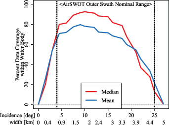
Figure 2. Approximately 70% of the AirSWOT radar data are recovered within the nominal swath range, with rapid data loss <4° and >17°. WSE data is present mostly at >4 degrees of incidence.
Download figure:
Standard image High-resolution image4.2. Comparison with in situ GPS
Of the 63 in situ WaSP GPS observations available, only 26 could be paired with AirSWOT matching the minimum water body size and AirSWOT data coverage. GPS observations [8] are strongly correlated with AirSWOT WSEs averaged across (250 m)2 areas around each GPS survey point [figure 3(A)]. However, a bias of approximately −58 cm (std.dev = 27 cm) is found between the two datasets, with AirSWOT WSEs lower than in situ WSEs. Overall, the full-resolution AirSWOT WSEs have a 1–2 meter elevation range within the (250 m)2 subset of the individual water bodies, further demonstrating the inherent noisiness of these WSE retrievals and the necessity for spatial averaging within water bodies to yield useful estimates of WSE. The supplement provides the statistics for all WaSP GPS—AirSWOT lake pairs [supplement table 1].

Figure 3. In (A), GPS elevations are sampled from 26 lakes across the ABoVE Domain and are correlated with AirSWOT WSE measurements (r2 = 0.999). While correlated, AirSWOT WSEs display a mean bias of −58 cm relative to GPS WSEs. Uncertainty analysis using leave-one-out and bootstrapping (20 000 iterations leaving out 1/4th of the data, with replacement) in (B) demonstrate the sensitivity of the bias estimate to the samples of the GPS data used. For leave-one-out and bootstrapping tests, the means are −57.9 cm and −58.2 cm. The 25th and 75th percentiles for leave-one-out are −58.3 cm and −57.6 cm, while bootstrapping are −59.8 cm and −56.8 cm. Density distributions of pixels with (250 m)2 open water areas for three representative lakes with in situ WaSP surveys are shown (in (C) and (D)) highlighting the noisiness in the data, having a range of up to two meters from the mean. The GPS measurement is represented by a black vertical line while the mean AirSWOT measurement is shown in red.
Download figure:
Standard image High-resolution image4.3. Comparison of AirSWOT WSE with LVIS WSE
Via comparison with in situ WaSP GPS, the LVIS RH65 elevation data were determined to be the closest approximation of the GPS WSE [figure S3]. Using the LVIS RH65 product, the average of the pixel-to-pixel differences between LVIS RH65 WSEs and AirSWOT WSEs yields a mean error bias, with AirSWOT WSEs 63 cm lower than LVIS. The results of the AirSWOT-LVIS mean error plotted against incidence angles are shown in figure S5. As reported in previous studies [9, 10], we find a strong relationship between incidence angle and absolute error (figure 4).

Figure 4. Relationships between the mean absolute error derived from the difference between AirSWOT WSE and LVIS WSE and the AirSWOT radar products pixel-to-pixel comparison provide four distinct filtering boundaries on the AirSWOT radar products: Incidence, Coherence, Magnitude, and Elevation Uncertainty. The filtering boundary of desired data is shown as a black line with directional arrows. A red local regression line shows how the absolute error decreases or increases with changing radar parameters. The scatterplot is represented as a smoothed point cloud demonstrating the density of points; points are tightly clustered where the point cloud is dark blue, and sparse where the cloud is light or white.
Download figure:
Standard image High-resolution imageFiltering recommendations can be made by identifying which incidence angles reduce the standard deviation and mean absolute errors. Relationships between mean absolute error and incidence angle, coherence, backscatter, and elevation uncertainty in the radar products suggest how to achieve WSE with higher accuracy and precision, reducing the noisiness seen in figure 3.
Figure 4 demonstrates absolute error relationships with the AirSWOT radar products, with positive correlations with elevation uncertainty and incidence angle, and negative correlations with magnitude and coherence. It is recommended that AirSWOT ABoVE 2017 data users isolate data where the elevation uncertainty is less than 1 meter, magnitude is greater than 5 dB, the incidence angle is between 5 and 15 degrees, and the coherence is greater than 0.8. These filtering recommendations provide insight into the spread of error values and into how precision and accuracy can be improved. Filtering the data reduces the bias in the pixel-based analysis from −63 cm to −54 cm. Bias correcting the data by adding 54 cm produces a mean absolute error (MAE) of 35 cm.
The reported bias is slightly different for spatially averaged lakes. Users are advised to spatially average AirSWOT WSE data to reduce noise, arriving at a single mean WSE value. Applying the filtering recommendations and removing pixels for which the absolute difference from the reference MERIT DEM is higher than 5 m, we extract AirSWOT WSEs from lakes larger than (250 m)2 and average the lake elevations, producing 1043 LVIS-AirSWOT lake coverage pairs across the entire domain. While the 1043 AirSWOT—LVIS lake pairs are correlated, scattered outliers greater than 20 meters skew the mean error between the two datasets to −88 cm (figure 5). As the pairs are within 1 m about 80% of the time, the 805 lake pairs having a mean WSE error of −45 cm (blue in figures 5(A) and (B)), can be used in further temporal analysis. Adding 45 cm for bias correction produces an MAE of 27 cm.
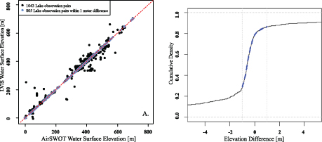
Figure 5. Black dots in (A) and line in (B) show AirSWOT vs. LVIS WSE after adding the MERIT reference elevation filter, using all 1043 available AirSWOT-LVIS lake observation pairs. Blue dots (A) and line in (B) show AirSWOT WSE vs. LVIS WSE after reference elevation filtering and limiting the absolute difference between AirSWOT and LVIS to 1 meter using 805 available AirSWOT-LVIS lake pairs.
Download figure:
Standard image High-resolution image4.4. Sub-seasonal variability in WSE
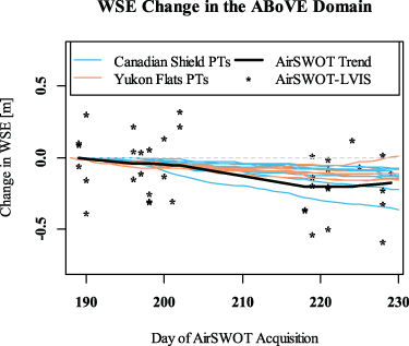
Finally, we assessed WSE changes mapped by AirSWOT and LVIS WSE over time [figure 6]. To summarize regional and sub-seasonal variability, AirSWOT-LVIS lake differences are aggregated into 29 sub-regional clusters based on the grouping of the AirSWOT flight lines (figure S2 shows the flight lines for the Peace-Athabasca region). Similarly, AirSWOT-AirSWOT WSE pairs can be used for this analysis, although errors inherent in the lakes used in the pairing cannot be normalized, amplifying the uncertainty in the sub-seasonal water level assessment. A previous study of summer 2017 lake variation demonstrated shrinking lake areas between July and August [24], corresponding to a seasonal drawdown of lake water storage. Eighteen pressure transducers (PTs) placed in lakes ranging from the Yukon Flats, Alaska, to the Canadian Shield demonstrate thesub-seasonal hydrological drawdown between July 6 and August 19, 2017 (day-of-year 187–231). Despite the spread in aggregated WSE elevation differences in lakes present in the time-series analysis represented in figure 6, there is a trend in the elevation difference between AirSWOT and LVIS, aligning with the change in water surface elevation from PTs. During this time, WSEs from PTs decreased by 7–35 cm, while AirSWOT shows a mean WSE decrease across the region of 17 cm.
Figure 6. After bias correction (see figure 5), spatially-averaged AirSWOT WSEs reveal a broad-scale drop in lake levels averaging ∼17 cm across the ABoVE domain over the period July 8–August 17, 2017. This finding is consistent with in situ time series of WSE acquired by 18 pressure transducers (colored lines: July 6- August 19, 2017). The 805 LVIS-AirSWOT lake pairs (from figure 5) have been aggregated into 29 regions (black dots). Reference datum (0 m) is relative to LVIS WSEs acquired in early summer.
Download figure:
Standard image High-resolution image
5. Discussion and conclusion
This study demonstrates the spatial and temporal capabilities of AirSWOT to map Arctic-Boreal lake WSEs and their sub-seasonal changes over time, as well as strengths and limitations of AirSWOT data collection and analysis across a >22 000 km2 region of the North American Arctic-Boreal region. AirSWOT radar retrievals of WSE across the ABoVE domain [16] were evaluated using precise in situ GPS measurements acquired by WaSP [8], in situ pressure transducers [24], and LVIS airborne LiDAR data [31]. For AirSWOT WSE retrievals to be beneficial to both hydrologic science and SWOT validation goals, its spatially-averaged values must meet or exceed SWOT elevation mean absolute error requirements of 25 cm for water bodies (250 m)2 and 10 cm for (1 km)2 water bodies [13]. AirSWOT radar should also secure useable returns over open water bodies. In support of ABoVE hydrology goals, AirSWOT WSEs should be able to capture Arctic-Boreal water storage changes. The immense ABoVE dataset presented here is thus a significant opportunity for both Arctic-Boreal hydrologic science and pre-launch SWOT mission planning.
A missing data analysis [figure 2] confirms that forward, specular scattering increases with higher incidence angles in flat water bodies [32], reducing the amount of backscatter returned to the AirSWOT radar sensor at incidence angles greater than 17°. However, missing data do not necessarily preclude retrieval of useful WSE measurements, as remaining data are still useful for estimating the WSE. Seemingly low data presence does not necessarily signify that entire water bodies are missing, but rather that fractional returns from water result in reduced data availability for spatial averaging and thus increasing the potential for error in WSE. To mitigate this problem in future AirSWOT campaigns, we agree [8] that increasing the overlap of flight lines would ensure areas experiencing specular scattering have multiple observations, more explicitly focusing on incidence angles greater than 17°.
Spatial averaging and various filtering techniques applied AirSWOT WSEs reduce noise and constrain random error in the WSE, reducing mean error biases ranging from −45 cm to −88 cm for observed water bodies. Possible bias sources include residual artifacts in the radar processing, signal delay, or solid earth tides [supplement 2]. Random WSE errors in the AirSWOT elevation product are reduced by applying the recommended filters of incidence angle (5–15 degrees), coherence (>0.8), magnitude (>5 dB), and elevation uncertainty (<1 meter) available in the accompanying products. Previous studies used similar filtering techniques as well as visual identification to select and manually remove regions of anomalous elevation values [26], while others automatically remove outliers based on an expected elevation range [28, 29].
Seasonal water storage change can be assessed by applying the filtering recommendations to AirSWOT flight lines and aggregating the AirSWOT-LVIS differences into 29 sub-regions across the ABoVE domain. Here, we identify an overall hydrologic drawdown of −17 cm across the ABoVE domain between July 8 and August 17, 2017, consistent with a −22 cm drawdown recorded with in situ pressure transducers installed in lakes across the ABoVE domain for AirSWOT WSE validation [24]. Using aggregated regions enables a seasonal water storage assessment, reducing the impacts of noise and errors found at the individual lake level. Because of residual errors in the WSE following filtering and spatial averaging, ABoVE AirSWOT data users are advised to examine multiple lakes or rivers (n > 50) in a given study area to identify relative changes in WSE rather than absolute elevations.
While our results suggest a large spread in mean error values across the ABoVE domain, previous studies of AirSWOT WSE focused on particular regions such as the Tanana River [26, 30], Yukon Flats [27], Willamette River [28], and the Mississippi River Delta [29]. As these examinations included the first AirSWOT datasets ever produced, JPL engineers were able to focus on these smaller regions to correct and re-process data as necessary, before the datasets were released to scientists. Unlike earlier studies, this study encompasses an immense region, covering 23 degrees of latitude and with 128 flight lines covering a 22 775 km2 area. Due to the size of the ABoVE collection, JPL engineers used more automation in preparing the data, significantly limiting manual corrections and multiple re-processing attempts before releasing the data. There have been multiple modifications and repairs made to the AirSWOT radar since 2014 due to it being an experimental instrument. As a result, slightly different product quality between studies and differences in reported error statistics across studies are expected. Future research directions for AirSWOT error analysis could include quantifying non-instrument sources of error, such as how water movement, wind, rain, and vegetation intrusion impact the AirSWOT radar signal, potentially contributing to errors observed across studies despite instrument changes.
Finally, we can answer the questions: How well did the AirSWOT radar map water surface elevations across the ABoVE domain? Can AirSWOT WSEs be used to measure storage change at seasonal time scales? We conclude 1) there is a correctable mean bias of −45 cm in the 2017 ABoVE AirSWOT collection relative to LVIS WSEs that was identified after filtering the AirSWOT elevation, 2) bias correcting the WSE data produces a mean absolute error of 27 cm, similar to the SWOT 'total height error' requirement of 25 cm for water bodies between (250 m)2 and 1 km2, and 3) AirSWOT can detect decimeter-scale water level changes over large regions. Through spatial averaging, vigorous filtering, and bias correction of AirSWOT WSE retrievals, small vertical changes in water surface elevation are detectable at the landscape scale, demonstrating the capacity of the AirSWOT data for broad-scale Arctic-Boreal hydrologic mapping and SWOT validation purposes.
Acknowledgments
The 2017 ABoVE AirSWOT data was processed using software developed at the Jet Propulsion Laboratory; we would like to thank the author of the InSAR software, Xiaoqing Wu, for contributing to the production of the data and supporting this study. GPS devices were provided by UNAVCO (formerly the University Navstar Consortium), and the GPS Precise Point Positioning (PPP) solutions were processed by researchers at the Centre National d'Etudes Spatiales (CNES). A portion of this work was performed at the Jet Propulsion Laboratory, California Institute of Technology, under contract with NASA. This work was funded by NASA Terrestrial Ecology Grant NNX17AC60A and NASA SWOT Science Team Grant NNX16AH83G.
Data availability statement
The data that support the findings of this study are openly available at the following URL/DOI: https://doi.org/10.3334/ORNLDAAC/1646.