


Abstract
A variance-maximization approach based on 19 years of weekly measurements of pollution in the troposphere carbon monoxide (CO) measurements quantifies the spatial-temporal distribution of global biomass burning. Seven regions consistent with existing datasets are discovered and shown to burn for longer, over a more widespread area. Each region has a unique and recurring burning season, with three dominated by inter- and intra-annual variation. The CO is primarily lofted to the free troposphere from where it spreads downwind at 800 to 700 mb with three exceptions: The Maritime Continent and South America where there is spread at 300 mb consistent with deep- and pyro-convection; and Southern Africa which reaches to 600 mb. The total mass of CO lofted into the free troposphere ranges from 46% over Central Africa to 92% over Australia. The global, annual emissions made using two different techniques lead to an increase of biomass burning CO emissions of 47TgCO/year and 99TgCO/year respectively. The larger increase is mainly due to two factors: first, a large amount of the emissions is lofted rapidly upwards over the biomass burning region and subsequently transported downwind, therefore not appearing near the biomass source in space and time and second, an increase in inter-annual variability. Consistently, there is an increase in variability year-to-year and during peak events, from which 35% to more than 80% of the total emissions is lofted into the free troposphere. The results demonstrate a significantly higher CO emission from biomass burning, a larger impact on the global atmospheric composition, and likely impacts on atmospheric chemistry and climate change.
Export citation and abstract BibTeX RIS

Original content from this work may be used under the terms of the Creative Commons Attribution 4.0 license. Any further distribution of this work must maintain attribution to the author(s) and the title of the work, journal citation and DOI.
1. Introduction
Biomass burning has been found all over the world due to agricultural burning, land clearing, and as a natural response to drought (Levine 2003, Malhi et al 2008). Due to the incomplete nature of biomass combustion, it contributes a significant fraction of the total global source of carbon monoxide (CO) emissions (Crutzen et al 1979, Crutzen and Andreae 1990). There has been a significant amount of work in the satellite era using measurements of fire radiative power and burned area (FRP & BA) as direct and semi-direct methods of measuring the spatial-temporal distribution of biomass burning (Olivier and Berdowski 2001, Wiedinmyer et al 2011, van der Werf et al 2017) and then constraining the mass emitted using in laboratory measured relationships (Bond et al 2004). These indirectly defined, bottom-up relationships, have been combined to demonstrate that over the past few decades, the total contribution of CO emissions from biomass burning has been significantly larger than in the pre-industrial past (van der Werf et al 2017).
However, there has not been a significant amount of work using in-situ measurements of CO to quantify changes in biomass burning. Studies have limited themselves to surface measurements (Delene and Ogren 2002), limited or non-spatially varying regions (Yu et al 2019), or seasonal, annual and other long-term average conditions (Duncan et al 2003, Jiang et al 2017, Buchholz et al 2018). However, recent large-scale biomass burning events are being highlighted in the news more frequently, leaving the impression that the phenomenon is recently changing (Nuh 2019, Sagita 2019a, 2019b).
One important factor with respect to constraining the emissions of CO from fires is that there is no generally agreed upon definition of what are appropriate bottom-up conditions that constrain or define when and where to even look for a signal of CO emissions attributed to biomass burning, with significant differences in meaning between such terms as biomass burning, forest fires, natural fires, agricultural fires, rubbish fires, biomass, etc (Syphard et al 2017, Lin et al 2019) For this reason, a top-down approach, where one relies on measurements of CO in the environment, could provide the basic statistics and a method by which those regions actually producing a significant amount of biomass burning CO emissions over a sufficiently long period of time can be classified (Cohen 2014, Cohen et al 2017). Recent work has found a significant amount of biomass burning is occurring in regions which are not observed to be burning using the standard FRP and/or BA approaches (Buchholz et al 2018, Deng et al 2019). This shows the value of top-down methods when questions are ill-posed or otherwise not readily constrained from a bottom-up perspective (Prinn 2004, Cohen et al 2011, Cohen and Wang 2014, Cohen 2014).
Since fires co-emit heat and aerosols with CO, a significant fraction of aerosol plumes have been found to rise above the surface, with some breaching the boundary layer (Val Martin et al 2018, Cohen et al 2018). Given that CO is water insoluble, it is expected that the vertically transported fraction should be at least as much as aerosols, given that any in-situ cloud formation will not enhance removal (Tao et al 2012). Othere recent studies have used monthly averages and statistical smoothing techniques on one hand, or non-linear chemical, physical, and dynamical models on the other hand to reduce the variability related to thes issues, and therefore have been able to eliminate the most significant forcings effects, allowing for higher detail at a loss of borader application (Zheng et al 2018, 2019). However, little research can presently be found addressing this point in an unbiased and comprehensive manner, in specific with an emphasis on extreme events and in a way that does not reduce the non-linearity, although a few studies have demonstrated that CO can spread farther downwind than co-emitted aerosols (Cohen and Prinn 2011).
We apply a simple variance maximization approach to the vertically resolved, weekly measurements of pollution in the troposphere (MOPITT) CO over a 19-year period from 2000 to 2018 to constrain and quantify the spatial-temporal distribution and magnitude of biomass burning. Comparison with existing datasets demonstrate the consistency of our findings near the surface. Using three different measures, we quantify the burning source regions, the vertical distribution over the source regions, and the flow downwind. Finally, we quantify the contribution of biomass burning CO to the whole atmosphere. Based on our knowledge, this approach has never been attempted before.
2. Data and methods
This study analyses the global-scale vertical distribution of CO as measured by MOPITT, with an emphasis on those regions changing most rapidly. These are the regions generally found to be dominated by biomass burning (including annual events, and variations occurring on an inter-annual and/or intra-annual basis), urban areas undergoing significant changes in their CO emissions profiles, or regions heavily impacted by the long-range transport of CO plumes.
2.1. MOPITT measurements of CO
We use remotely sensed CO measurements retrieved from the MOPITT instrument aboard the Terra satellite, which has collected data from March 2000 to the present (Drummond et al 2010, 2016). Specifically, we use the day time only retrieval (since night time data contain more bias) version 8, level 3, joint thermal infrared and near infrared (Deeter et al 2013, 2017). To constrain the vertical CO distribution we further use both the CO mixing ratio profile and the degree of freedom signal (DFS).
We specifically employ the DFS to constrain over which levels there exists vertical resolution. The DFS represents the number of vertical levels from which the concentration profile can be reasonably discerned within the total column. The DFS should be considerably larger than 1 to imply there is more than one layer of the atmosphere significantly contributing towards the total column weighting. There is no clear guideline in the literature as to what number to use and therefore we select a value of 1.5, which we demonstrate provides a significant amount of coverage globally for regions found to be important in this work, allowing for two significant yet overlapping layers (i.e. between the surface, lower free troposphere, and/or the tropopause). Additionally, this cutoff yields a sufficient amount of data to draw statistically significant scientific insights.
There has been work demonstrating a limited amount of sensitivity in terms of the reliability of the vertical profiles to represent actual CO as compared to the a priori model derived CO used in the retrieval (Worden et al 2010). This issue is relevant in the case of this work, since we are identifying and quantifying sources of CO which have not been previously identified or have been underestimated, and hence are not well represented by the current a priori. Following the retrieval equation (equation (2) in Worden et al 2010) we have computed the row-sum of the retrieval matrix for each weekly set of values and plotted them in (figure S1 (stacks.iop.org/ERL/15/104091/mmedia)). As observed, the value is very close to 1.0 (and thus the contribution from the model a priori is approximately 0.0) over each of our spatial-temporal regions identified in this work. Furthermore, over our regions, the value moves closer to 1.0 during the biomass burning times identified in our work, indicating that the CO is based on atmospheric retrievals of actual CO. The fact that there are multiple levels which contribute to the retrieval is not surprising, just a clear demonstration that our results provide an additional value, that the improvment of the a priori should provide additional benefit for downstream users of MOPITT data in relation to bioamss burning.
2.2. Global fire emissions database (GFED)
GFED provides an estimate of the fire emissions of carbon by combining satellite measurements of BA and vegetation productivity (van der Werf et al 2017, Akagi et al 2011, Giglio et al 2013). We employ GFED4s version in this work (van der Werf et al 2017), specifically using the mapped biomass burning total carbon emission as the reference for the true location of surface biomass burning. We use the GFED monthly emissions product from 2000 to 2018 including 'beta level' data for 2017 and 2018, and aggregate the data to 1° by 1° to be compatible with MOPITT.
One approach to select those regions with a significant amount of burning is based on setting a high cutoff from 2000 through 2018. In specific, we consider an average value of 10 g m−2 year to be highly burning (total emission of 190 g m−2). However, there are certain gap-years in the data, in which case we require a larger amount of emissions in other years to compensate, defining those regions with a three-year running-sum greater than 30 g m−2 to be highly burning regions (figure 1(a)). This allows those regions which burn frequently (although still considering those regions in which special atmospheric phenomenon may prevent annual burning), as compared to one or two-off events, to be considered in this work.

Figure 1. (a) GFED total carbon emissions (g m–2) from 2000 to 2018 over high fire regions (cutoff is based on a three-year running local sum of 30 g m−2); (b) Spatial distribution of the normalized standard deviation of the MOPITT CO surface level concentration (DFS > 1.5); and (c) Biomass burning regions constrained where the normalized standard deviation of the MOPITT CO surface concentration is larger than 0.30 (land only, 60°S < Latitude < 60°N). The regions in this paper [and abbreviations] are displayed in red boxes (first top to bottom, next left to right): Central America [CAM], South America [SAM], Central Africa [CAF], Southern Africa [SAF], Continential Southeast Asia [CSEA], the Maritime Continent [MC], and Australia [AUS].
Download figure:
Standard image High-resolution imageThis approach yields results consistent with known seasonal burning located in Central America, South America, Central Africa, Southern Africa, Continental Southeast Asia, The Maritime Continent, and Northern Australia. However, this approach also yields a small number of relatively small high biomass burning regions over some high latitude areas, including Canada, Eastern Europe, and Russia. However, MOPITT CO measurements have a weak sensitivity or a lack of data availability over these high latitude areas, and therefore we do not include these regions further.
2.3. Statistical techniques and methods for selecting highly variable regions/biomass burning regions
The variance of CO is a useful tool to understand regions which are frequently undergoing rapid changes or are significantly changing their characteristic over decadal time scales. To account for regions which have a significant fraction of change coupled with a low mean, we compute the normalized standard deviation (figure 1(b)), defined as the standard deviation divided by the mean. The regions of the world with the highest normalized standard deviation are found in Central America, South America, Central and Southern Africa, Continental Southeast Asia, and the Maritime Continent. Most of these regions are known to be significantly influenced by biomass burning, with a relatively low CO loading most of year, but very high loading of CO over a short time frame during the biomass burning season (Cohen 2014). However, this approach cannot capture those biomass burning regions very well where there is a low amount of continuous burning throughout the year, because these regions wind up with a very small relative change over time and space, and tend to be classified as urban regions (Lin and Cohen ). Here, our purpose is to find a best cut off for the normalized standard deviation to quantify the biomass burning geographical fit between the MOPITT CO concentration at the surface and the GFED high fire regions.
The normalized standard deviation of the MOPITT CO concentration at the surface is tested in steps of 0.01 from 0.20 to 0.35 to ensure the results are consistent over land (excluding the possibility of significant offshore burning). Those regions with a high standard deviation over the ocean adjacent to a continent are almost certainly due to long-range transport from the adjacent land-based location. We compare our regions classified by the various cut offs to those based on GFED, with the geographical boundaries given in (figure S2) and (table S1), and find that the cut off of 0.3 yields the most similarity (figure 1(c)).
3. Results
3.1. Constraining biomass burning regions over different pressure levels
We compute the value at the surface because the actual emissions from biomass burning are generated at the surface. However, to account for the subsequent rapid adjustment as a function of the heat co-emitted with the CO and other meteorological factors impacting any vertical transport, we need to also analyze in the vertical. We therefore further apply the cut-off procedure to each MOPITT CO mixing ratio profile in the Troposphere from 900 mb to 300 mb (figures 2(a)–(g)). The rationale is to test which regions at each height have the same spatial characteristics as those which meet the biomass burning definition over both the total column and the surface measurements in this work. While in general there should be very little directly lofted to 300 mb, it has been demonstrated that occasionally organized deep convection (Ekman et al 2011) or pyroconvection (Yu et al 2019) are capable, and therefore we want to test these possibilities consistently.

Figure 2. Biomass burning emission regions constrained by normalized standard deviation greater than 0.30 on eacah layer from 900 mb to 300 mb at 100 mb intervals (a to g respectively).
Download figure:
Standard image High-resolution imageWe find that the respective biomass burning geospatial region on each pressure level has a different distribution as compared to the underlying surface level. This spread is due to differences in large-scale meteorology, fire forcing, local dynamics, and in-situ atmospheric heating and cooling due to co-emitted aerosols (Wang et al 2020), and as such is found to be unique in the different biomass burning regions, although there are many similarities. First, the geospatial distribution is wider above the surface, particularly so from 800 mb to 700 mb, although in a few cases the perturbed area can be observed up to 300 mb (figure 2). These results are consistent with the case where heat co-emitted with the fire lofts a fraction of the CO directly into the lower free troposphere, where is subsequently spreads further downwind due to a slower chemical loss rate (Prinn et al 1987) and a generally faster wind speed. However, the direction of the wind also changes with height, leading to a spread that may occur over different directions at different heights. To ensure that we are looking at the impact from the fire source, we discard those layers which do not have a complete overlap with the surface geospatial region, since on the weekly time scales used here, the buoyancy generated from the fires and other associated fire-induced effects have a sufficient amount of time to transport the mass in the vertical.
3.2. Maximum spread area
We note the vertical layer with the greatest geospatial area impacted by the biomass burning (here after the maximum spread area), and use this later to approximate the mass exported. We find that the maximum spread area is 800 mb over Central America and Australia, 700 mb over South America, Central Africa, Southern Africa and Continental Southeast Asia, and 300 mb in the Maritime Continent. Along with the maximum spread area, we can approximate the overall impact by knowing the maximum height to which the plume spreads (plume cap). The plume cap is found to be 700 mb over Central America, Central Africa and Australia, 600 mb over Continental Southeast Asia, 500 mb over Southern Africa, and 300 mb over South America and the Maritime Continent.
3.3. Correlation/overlap
We propose a test of the correlation between the temporal variation of the CO concentration averaged over the surface geospatial region, with that of the CO concentration at every level in the vertical above the surface (hereafter called the correlation/overlap approach) (table 1). The rationale is to ensure that the timing and magnitude of the CO at height matches that at the surface where the fires are originating. This ensures that the results are actual observations of the CO plume rise, not just a random perturbation in the local air aloft. We expect the correlation between CO concentration at the 900 mb and the surface level to be extremely high, since the CO at 900 mb is frequently on a weekly time scale mixed in the boundary layer (Guo et al 2019), especially so in the convective boundary layer (Zhang et al 2018, Lou et al 2019).
Table 1. (top) Correlation (R) between the CO concentration on the surface level and on the respective pressure levels (horizontal); and (bottom) Pseudo-mass percentage on each respective pressure level and the total percentage in the free troposphere (800 mb to 300 mb) (horizontal). For all cases, the biomass burning regions are given in the (vertical), and slashes denote levels where there is no data available.
| Correlation with 1000 mb | 900 mb | 800 mb | 700 mb | 600 mb | 500 mb | 400 mb | 300 mb | ||
|---|---|---|---|---|---|---|---|---|---|
| Central America | 0.95 | 0.91 | 0.85 | ||||||
| South America | 0.96 | 0.89 | 0.85 | 0.66 | 0.55 | 0.58 | 0.56 | ||
| Central Africa | 0.83 | 0.87 | 0.88 | ||||||
| Southern Africa | 0.97 | 0.85 | 0.84 | 0.75 | 0.59 | ||||
| Continential Southeast Asia | 0.83 | 0.86 | 0.82 | 0.69 | |||||
| Maritime Continent | 0.82 | 0.55 | 0.59 | 0.57 | 0.52 | 0.45 | 0.33 | ||
| Australia | 0.73 | 0.51 | 0.72 | ||||||
| Pseudo-mass percentage | 1000 mb | 900 mb | 800 mb | 700 mb | 600 mb | 500 mb | 400 mb | 300 mb | Total 800 mb to 300 mb |
| Central America | 23% | 26% | 32% | 19% | 51% | ||||
| South America | 17% | 17% | 17% | 15% | 12% | 6% | 6% | 11% | 67% |
| Central Africa | 31% | 23% | 23% | 23% | 46% | ||||
| Southern Africa | 13% | 12% | 21% | 23% | 18% | 13% | 75% | ||
| Continential Southeast Asia | 23% | 20% | 28% | 23% | 6% | 57% | |||
| Maritime Continent | 8% | 6% | 2% | 7% | 17% | 17% | 18% | 25% | 86% |
| Australia | 1% | 7% | 80% | 13% | 92% |
This result is a critical step to ensure that we have accounted for the changes in the CO loading that could be impacted by local forcings including terrain, dynamics, convection, and aerosol-radiative feedback (Tao et al 2012, Li et al 2017) or random perturbations as a result of long-range transport from elsewhere (Price et al 2004). To be conservative, we roughly look for those regions which have at least one third of their total variation (i.e. 17 weeks a year or less) explained by the surface biomass burning perturbations, or a coefficient of correlation of R > 0.58. This is more than sufficient, given that the biomass burning duration over most biomass burning regions of the world using our approach is less than 12 weeks a year (Guo et al 2017). Results of the correlation/overlap approach show that the level of maximum biomass burning CO transported to occurs at 800 mb over Central America, South America, and Continental Southeast Asia, both 800 mb and 700 mb over Central Africa and Southern Africa (although the timing of the burning occurs during different months in these two regions), and 700 mb over the Maritime Continent and Australia.
We take a further step to understand the temporal variation over the biomass burning regions at height by analyzing the time series as a function of height (figure S3). At the surface, the median CO concentration is generally very low, ranging from 101 ppbv to 257 ppbv. However, the measurements experience an extremely high value during the short period when the biomass burning occurs, with the maxima ranging from 315 ppbv to 813 ppbv. We observe clearly that the temporal patterns at each level are consistent with each other and the surface during the peak times, supporting that the variation is due to the spike generated by the biomass burning, as compared with random noise or another event that occurred off-season from the biomass burning. We further determine that the magnitude of the results is much larger than any bias in the retrievals as given in (figure 12 of Deeter et al (2019)) and therefore are valid throughout the remainder of this paper.
We find that while a significant amount of the variation is due to the annual biomass burning peak, there is also an important component due to intra-annual and inter-annual variation. For example, in some years the biomass burning CO has a significant impact in South America at the 300 mb level, such as in 2005, 2007 and 2010, but in other years it is not detected at all at 300 mb although it is clearly present in the lower free troposphere, such as in 2000, 2001, 2003, 2008, 2009, 2011, 2013, 2014, 2016, 2017 and 2018. In the case of Southern Africa, the variance has an important contribution from the fact that the biomass burning rises to the upper atmospheric layers only during the larger of the two annual fire events, but not during the smaller annual event. In the Maritime Continent, the total number of years with a significant amount of biomass burning is low, but the el-Nino years when it occurs (2006 and 2015) make it the most significant globally with concentration peaks of about 740 ppbv and 810 ppbv at the surface and 170 ppbv and 250 ppbv at 300 mb. However, the Maritime Continent also is a significant source in 2002, 2004, and 2014, although not as much as in 2006 and 2015.
We use the regions found from the correlation/overlap results in combination with GFED emissions to compute a new three-dimensional biomass burning CO emissions product, with a weekly time resolution. First, the regions in space and time that overlap between weekly-interpolated GFED emissions and the correlation/overlap approach, are used to form an emissions to loading ratio E/L (equation (1)) where E is the GFED emissions [g m−2] and L is the MOPITT CO column loading [molecules cm−2]. Next, this value is multiplied by the weekly column loading over the entirity of the correlation/overlap region to obtain an estimate of the emissions (equation (1)). The statistics of the resulting emissions are given in table 2, with the weekly time series given in (figure S4).
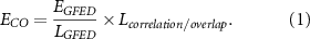
Table 2. Annual average emissions of biomass burning CO [TgCO/year] computed based on: GFED [GFED]; the correlation/overlap approach and (equation (1)) [C/O]; and the enhancement to the CO biomass burning mass computed using the pseudo mass approach and (equation (2)) [P/M]. In the case of P/M, the annual average emissions for the various grouped or individual pressure levels is given in parentheses (). In all cases, due to the precision of the underlying data, results have only two significant digits.
| GFED | C/O | P/M 1000–300 | P/M 800–300 | P/M 1000 | P/M 900 | P/M 800 | P/M 700 | P/M 600 | P/M 500 | P/M 400 | P/M 300 | |
|---|---|---|---|---|---|---|---|---|---|---|---|---|
| AUS | 1.6 | 1.7 | 4.7 | 4.1 | 0.11 | 0.55 | 2.6 | 1.5 | ||||
| CAF | 48 | 53 | 8.2 | 5.2 | 1.7 | 1.3 | 2.6 | 2.6 | ||||
| CAM | 4.6 | 6.5 | 2.3 | 0.86 | 0.62 | 0.79 | 0.86 | |||||
| CSEA | 13 | 17 | 9.0 | 6.7 | 1.4 | 0.92 | 3.2 | 3.0 | 0.53 | |||
| MC | 46 | 56 | 8.7 | 7.0 | 0.90 | 0.78 | 0.19 | 0.63 | 1.5 | 1.6 | 1.5 | 1.6 |
| SAF | 110 | 107 | 34 | 28 | 2.9 | 2.4 | 5.1 | 8.0 | 6.7 | 3.8 | 2.5 | 2.2 |
| SAM | 38 | 68 | 32 | 19 | 6.6 | 6.2 | 5.8 | 5.5 | 2.8 | 1.3 | 1.4 | 2.0 |
| GLOBAL | 262 | 309 | 99 | 71 | 14 | 13 | 20 | 21 | 11 | 6.7 | 5.4 | 5.8 |
Over all of the regions studied, except for Southern Africa, there is an increase in the annual CO emissions using the correlation/overlap method, with a gobal total increase of 47TgCO/year. However, this increase masks the fact that there are some differences in the timing and spatial extent, leading to an increase in the 12th percentile of emissions (which corresponds to the second highest annualized week-by-week difference) at all sites, with three regions showing a very large increase during the peak season: 0.58TgCO/week in Central Africa, 0.71TgCO/week in the Maritime Continent, and 1.2TgCO/week in South America.
3.4. Pseudo-mass ratio
Next we approximate the total CO pseudo-mass exported in the vertical over each biomass burning region by multiplying the temporal mean CO concentration at each vertical level by the maximum spread area at each vertical level. These values are summed and normalized as a fraction of the total sum in the vertical over each region, yielding the percentage of the CO pseudo-mass at each level (table 1). The first result is that each region has a minimum of 46% to a maximum of 92% of the total mass associated with the biomass burning lofted to the free troposphere. It is important to note that these values are likely biased low in terms of the vertical transport, since we are using the mean over the entire month, not solely the biomass burning maximum time.
The heights to which the maximal amount of CO lofts using this approach is sometimes different from the correlation/overlap approach. We find similar results between the two methods in Central America 32% (19%) and Continental Southeast Asia 28% (23%), with a respective percentage of CO mass transported to and spreading respectively first at 800 mb and (second at 700 mb). We also find similar results between the two methods in both Central Africa 23% (23%) and Southern Africa 23% (21%), with a respective percentage of CO mass transported to and spreading respectively first at 700 mb and (second at 800 mb). A significant difference between these two regions is that Southern Africa has 18% of mass exported at 600 mb, whereas Central Africa has none. In the case of South America, we find a similar result between the two approaches at 800 mb where 17% of the mass is transported to, but a significantly different result in that 11% is also transported to 300 mb, while the correlation/overlap approach does not yield a significant value. The results of this approach are also different for both the Maritime Continent where 25% of the mass is transported to and spreads at 300 mb, and 77% of the mass is transported to and spreads at 600 mb to 300 mb, and in the case of Northern Australia where 80% and 13% of the total mass is lofted to and spreads at 800 mb (which the correlation/overlap approach did not show was significant) and 700 mb respectively.
The temporal and spatial results over the surface layer and the two in-situ layers of maximal transport (where there is agreement between the correlation/overlap and pseudo-mass approaches) or the optimal height from each approach (where there is not agreement) are found to be consistent. First, the respective time series capture both the timing and duration of the peaks consistently across all of the regions at the levels as determined (figures 3(a)–(g)). Next, there is a complete overlap of the surface region by each of the respective maximum spread areas for each of the corresponding regions, which we have displayed at the respective levels of 800 mb, 700 mb, 600 mb, and 300 mb (figures 3(h)–(k)).

Figure 3. Time series of average CO concentrations (ppbv) at the surface and each regions' respective significant vertical levels to which the respective biomass burning CO has been lofted (a-g); Comparison of the biomass burning emission spatial regions on surface and at the respective significant pressure levels (60°S < Latitude < 60°N) (h-k).
Download figure:
Standard image High-resolution imageAs can be clearly noted from these figures, the size of the spread is always larger in the free troposphere than at the surface, although the direction of spread is strongly mediated by the prevailing winds. It is interesting to note that a significant amount of this downwind transport occurs over the ocean throughout most of the world, except for in Asia, where a significant amount is transported over heavily populated regions downwind. In consideration of the possibility that the vertical rise is controlled by changes in the large-scale circulation are the same times that these mass changes are occurring, we checked the state of the large-scale atmospheric divergence at 925 mb, and found that other than South America, the rest of the regions are below the world average divergence at this level (figure S5). Even in South America, the divergence is only slightly above the global avereage, and is still a factor of 2 lower than over regions of large scale subsidence or lofting. Finally, recent work by Wang et al (2020) has shown that using simple relationships between FRP, the thermodynmic condition of the atmosphere, and the vertical velocity still may be inferior to using the column magnitudes of CO and NO2 in tandem, further lending support to our approach used here.
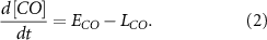
We use the time series of psuedo mass (figure 3) in combination with the atmospheric mass conservation equation (equation (2)) to solve for the emissions of CO (actually: emissions minus chemical production/loss, or ECO—LCO). The statistics of the annual average emissions, level-by-level from 1000 mbar to 300 mb, and summed both over the total atmosphere and the free troposphere are given in table 2. The weekly time series for the total atmospheric and free troposphre emissions, as well as a comparison of GFED emissions are given in (figure 4).

Figure 4. Time series of weekly CO Emissions (TgCO/week) computed using the pseudo mass and equation (2). For all plots, the x-axis represents the weeks from 2000 to 2018 and the y-axis represents the Emissions (TgCO/week). Blue circles are GFED emissions, red squares are the total atmospheric emissions from the pseudo mass approach and equation (2), and green stars are the total emissions in the free troposphere (800–300 mbar).
Download figure:
Standard image High-resolution image
Over all of the regions studied, there is a significant increase in the annual average CO emissions using the pseudo mass method, with a region-by-region increase ranging from 1.9TgCO/year in Central America to 28TgCO/year in South America, an a total global increase of 99TgCO/year.
However, this increase masks two significant and important factors. First, that the large majority of the increase in emissions is due to emissions above the surface. Australia, Central America, Continential Southeast Asia, and South America all have a similar amount of emissions within the boundary layer and overall, while and Central and Southern Africa (up to 800 mb) and the Maritime Continent (up to 500 mb) have some amount of their vertical emissions represented by the results from the correlation/overlap approach. This indicates that the important difference is the enormous amount of mass emitted into the free troposphere that is not currently captured by GFED and the correlation/overlap approach (figure 4). The second issue is that the inter-annual variability and the emissions at the peak times both differ by quite a large amount as compred to GFED, with the 12th percentile of emissions at all sites showing a very large increase, ranging from 0.15TgCO/week in Central America, to 2.3TgCO/week in Southern Africa.
4. Discussion
The results obtained using the two approaches are found to be higher than many other biomass burning estimates in the literature on average, they are certainly not outside their upper bound over the spread of different models. The underlying measured concentrations in this work have also have not been adjusted downward to compensate for 'model deficiencies' as is a generally adapted technique when working with biomass burning emissions of CO as described in Lamarque et al (2010, figure 8). The CO emissions computed over the 30-year biomass burning period from 1980 to 2010 across different models (Granier et al 2011, figure 6) show a range from 15TgCO/year to 230TgCO/year in South America and a range from 70TgCO/year to 270TgCO/year in Africa, which is lower than the annual global average CO emissions of 68TgCO/year and 160TgCO/year in the same respective regions. The highest years recorded are focused on the 1997 El-Nino and its 1998 aftermath, and have a range from 450TgCO/year to 650TgCO/year, which implies an enhancement of roughly 10% over each of these peak years due to the Pseudo-Mass calculated emissions of 63TgCO/year in Africa (2015) and 42TgCO/year in South America (2007) for the respective highest years on record.
The abnormally higher estimated emissions are obtained using the due to three specific reasons acting in tandem with each other, which in general bottom-up approaches or the correlation/overlap approach cannot typically consider, since they are limited to the well-defined area that the biomass burning occurs in, and to relationships formed from small sample sizes. First, a large amount of the total emissions is rapidly transported above the bounGdary layer in the vertical, from where it is rapidly transported downwind and away from the biomass burning region. Second, local cloud cover, smoke cover, and sources outside of the swath width can still be measured due to downwind transport or using weekly scale aggregated data. Third, there is a very large amount of inter-annual and intra-annual variability which is not picked up at monthly scales and both aerosols and cloud cover further cause data loss at daily scales, therefore leading to less ability to reproduce particularly short but intense or atypical emissions conditions.
This magnitude of increased emissions is not out of line with increased emissions of BC from top-down studies such as Cohen and Wang (2014) but overall may have significant impacts. The first issue is that ultimate emissions of CO2 may be larger than thought due to more conversion from CO than previously assumed, while at the same time being much harder to measure with the new generation of CO2 satellites, since they have a narrow swath and will not pick up the downwind transport well. Secondly, the extra CO in the atmosphere will impact upon the OH radical and hence lead to a change in the lifetime of CH4, which itself is another controversial topic at the present time. Thirdly, co-emitted species which follow a similar injection and downwind transport pattern may lead to more of a loading of the short-lived climate forcers BC and Ozone, as they spread further from source regions and increase their atmospheric in-situ lifetime.
There are a few uncertainties and limitations associated with this approach. First off, there may be some bias introduced due to rapid production of CO in-situ, which will tend to be between +2% and −5% (figures 8 to 11, Cohen and Prinn (2011)). Secondly, there may be an additional bias in the small subset of plumes that advect more than 1 week downwind, of up to 8% for an extra week in-situ. However, based on NCEP reanalysis wind speed, this may only have an impact on the 500 mb and 600 mb levels over South America and the Maritime Continent. Third, there are uncertainties in the CO measurements themselves, which may be as high as 30%. A fourth issue is the limitation due to the assumption of what exactly constitutes the biomass burning start and end time, as compared to the background conditions of the pseudo mass assumption. In this case, a two standard deviation filter with four passes was used, and the results are definitively conservative (Cohen and Prinn 2011). Finally, another limitation is that sources contributing fires but below the standard deviation ratio cutoff established in the first step, are likely not observed, whether they are due to slow changes in burning, or are burning occurring mixed in urban areas and yield a net signal profile more like that of an urban area, even though rubbish and trash burning are both known and significant sources. Similarly, due to the sparse amount of data, low data quality, as well as infrequent occurrance, fires from the Arctic regions are missed using this technique, introducing another low-bias in terms of these results.
5. Conclusions
We have applied a new technique to 19 years of MOPITT CO measurements to establish and understand the spatial, temporal, and vertical distribution of CO associated with biomass burning around the globe. The major biomass burning regions are found to burn with an annual or twice annual frequency, although there is significant inter-annual and intra-annual variation. In terms of the vertical distribution, over all of the major biomass burning regions of the Earth that frequently burn, a significant amount of the material is lofted above the surface and exported at different heights. Here we have quantified the temporal and vertical distribution of the magnitude of this transport.
First, most of the CO is lofted to and spreads at the 800 mb or 700 mb levels over most of the global biomass burning regions. This is supported by the maximum spread area approach at all sites except for the Maritime Continent, the correlation/overlap approach at all sites, and the pseudo-mass approach at all sites except for South America, Southern Africa, and the Maritime Continent. The divergence of the results over the Maritime Continent are consistent with each other in that there is a significant amount of CO lofting to and spreading at 300 mb, albeit only occasionally. In the cases of South America and Southern Africa, there is a secondary but still not insignificant amount lofting to and spreading respectively at 300 mb and 600 mb, also not annually, but more frequently than in the Maritime Continent. These findings are consistent with significant deep convection and inter-annual variation due to global-scale coupled atmosphere-ocean forcings that occur over these regions of the world.
Second, a minimum of 46% of the global biomass burning mass is transported into the free troposphere. Subsequently over all three source regions in Asia and Australia, the plumes advect downwind over land regions with a significant population, possibly leading to an impact on air pollution over.
Third, we have introduced two top-down approaches to estimate the emissions of CO, one based on correlation/overlap and scaling after using GFED and MOPITT for training, and the second based on a direct integration of the mass balance equation an pseudo mass. Both new emission datasets have a weekly frequency, with the latter also offering a vertical distribution of emissions. The magnitude of CO emissions is larger in both new emission cases, by an annual average of 47TgCO/year based on the correlation/overlap approach and 99TgCO/year based on the pseudo-mass approach. Both datasets match the measured inter-annual and intra-annual variation better, in terms of start and finish time, spatial extent of the emissions, and high and low years. The differences in the magnitude between the two different approaches are directly attributable to the large amount of CO observed in the free troposphere, with the latter approach lofting from a minimum of 37% to a maximum of 87% of the total emissions to 800 mb or higher.
These findings imply that the current FRP and/or BA techniques are leading us to severely underestimate the total amount of biomass burning emissions, and their subsequent impact on the composition of the atmosphere. We provide evidence to encourage the community to further consider and improve upon the current approach, by taking a more whole-atmosphere approach to understanding biomass burning.
Acknowledgments
We acknowledge the PIs of the NASA MOPITT, GFED (www.globalfiredata.org), and NCEP projects for providing the remote sensing measurements and data. The work was supported by the Chinese National Young Thousand Talents Program (Project 41180002), the Chinese National Natural Science Foundation (Project 41030028), and the Guangdong Provincial Young Talent Support Fund (Project 42150003). All data currently in supplements has been placed into the doi listed under 'data availability' or in http://doi.org/10.6084/m9.figshare.12472151.
Data availability statement
The data that support the findings of this study are openly available at the following URL/DOI: https://doi.org/10.6084/m9.figshare.11302229.