


Abstract
The future European electricity system will depend heavily on variable renewable generation, including wind power. To plan and operate reliable electricity supply systems, an understanding of wind power variability over a range of spatio-temporal scales is critical. In complex terrain, such as that found in mountainous Switzerland, wind speeds are influenced by a multitude of meteorological phenomena, many of which occur on scales too fine to capture with commonly used meteorological reanalysis datasets. Past work has shown that anticorrelation at a continental scale is an important way to help balance variable generation. Here, we investigate systematically for the first time the possibility of balancing wind variability by exploiting anticorrelation between weather patterns in complex terrain. We assess the capability for the Consortium for Small-scale Modeling (COSMO)-REA2 and COSMO-REA6 reanalyses (with a 2 and 6 km horizontal resolution, respectively) to reproduce historical measured data from weather stations, hub height anemometers, and wind turbine electricity generation across Switzerland. Both reanalyses are insufficient to reproduce site-specific wind speeds in Switzerland's complex terrain. We find however that mountain-valley breezes, orographic channelling, and variability imposed by European-scale weather regimes are represented by COSMO-REA2. We discover multi-day periods of wind electricity generation in regions of Switzerland which are anticorrelated with neighbouring European countries. Our results suggest that significantly more work is needed to understand the impact of fine scale wind power variability on national and continental electricity systems, and that higher-resolution reanalyses are necessary to accurately understand the local variability of renewable generation in complex terrain.
Export citation and abstract BibTeX RIS

Original content from this work may be used under the terms of the Creative Commons Attribution 4.0 licence. Any further distribution of this work must maintain attribution to the author(s) and the title of the work, journal citation and DOI.
1. Introduction
The European energy system is expected to change dramatically over the next 30 years with the phaseout of fossil fuels in order to meet 2050 carbon targets (Fragkos et al 2017). Key technologies poised to replace incumbent infrastructure are solar photovoltaics and wind turbines. Wind electricity generation capacity increased by 157.7 GW in the period 2000–2017 in the EU alone (Fraile et al 2018), and is expected to continue growing.
However, existing wind electricity generation capacity on the European continent is concentrated in the North Sea region (Staffell and Pfenninger 2016). On the current trajectory of wind farm deployment, large-scale weather patterns affecting the entire European continent (so-called weather regimes) are likely to cause large swings in wind electricity generation on subseasonal time scales of 10–60 d (Grams et al 2017). To ensure that wind farm electricity generation remains relatively constant on subseasonal time scales, Grams et al (2017) showed that it is important to consider greater wind turbine deployment in southern or high-latitude regions of Europe. Within this north-south regime performance divide, Swiss wind farms are expected to perform similarly to those in neighbouring, central European countries (Grams et al 2017). Consequently, Switzerland is currently not deemed capable of contributing to the smoothing of the European electricity system, nor exploiting the economic benefits that might emerge to incentivise such smoothing. However, Grams et al (2017) did not consider the country's complex terrain, simulating wind patterns at an aggregated country level based on a global meteorological reanalysis with ∼55 km horizontal resolution (Staffell and Pfenninger 2016).
Given its complex orography we would expect the spatio-temporal variability of wind in a country like Switzerland to be greater than suggested by nationally aggregated data. Indeed, studies with higher spatial resolution have shown this to be the case (Jafari et al 2012, Kruyt et al 2017). These studies show that the alpine range, Jura range, and the Swiss plateau all exhibit site-specific wind speed strengthening and suppression at time scales ranging from diurnal to seasonal. Valleys experience an increase in wind speed in the mid-afternoon, while crests experience the inverse: an increase in wind speed overnight followed by a decrease in the afternoon—referred to as mountain-valley breezes. On slightly larger spatial scales, complex orography favours channelling flows that persist for several hours to a few days. Well-known examples are (1) the easterly Bise when low-level winds are enhanced in the Swiss Plateau region due to channelling between the Jura range and the Alps and (2) the north-south oriented Föhn flow extending from specific alpine valleys into the foot hills and beyond (Federal Office for Meteorology and Climatology 2015). These local spatio-temporal patterns could represent both barriers and opportunities for wind farm deployment. For example, high afternoon output from valley-deployed turbines could exacerbate line loading in alpine regions, when hydroelectric power output is particularly strong (Singh et al 2014).
The patterns are evident both in measured and modelled data (Jafari et al 2012), but require a high model resolution to accurately simulate. Jafari et al (2012) required a 3 km resolution to achieve resemblance with measured data; a horizontal resolution of 9 km was already too coarse even to simulate daily or weekly averages. Generally, to account for terrain variance, past work suggests that simulations require a 2 km or finer resolution (Salvador et al 1999). This is particularly important in valleys at low heights above surface, where local differences in terrain effects and surface roughness will lead to large simulation errors if a low spatial resolution is used. Because of this, studies so far have been constrained to making conclusions either at specific measurement sites or on average across wider geographic scales, ignoring the more complex local patterns. Interpolating between known measurement sites is not an option since, unlike in low-lying countries, there is little to no correlation between sites as a function of the distance between them (Kruyt et al 2017).
The Consortium for Small-scale Modeling (COSMO) regional reanalyses may offer a solution by accurately modelling local variability of wind while still providing consistent long-term time series across wider geographic areas (Kaiser-Weiss et al 2019). Two versions exist: one with 2 km (COSMO-REA2) (Wahl et al 2016) and another with 6 km (COSMO-REA6) (Bollmeyer et al 2015) horizontal resolution. On flat terrain across Europe, COSMO-REA6 has been shown to accurately simulate wind speed (Borsche et al 2016, Frank et al 2019, Ramirez Camargo et al 2019), often with improved performance over COSMO-REA2 (Frank et al 2020, Ramirez Camargo et al 2019). Although Ramirez Camargo et al (2019) showed that the higher resolution COSMO-REA2 outperforms COSMO-REA6 in complex terrain, validation was limited to only two isolated measurement sites and without comparison to the underlying meteorology affecting wind speeds in the region. Thus it remains to be seen whether the high resolution of both COSMO reanalyses is sufficient to capture all expected meteorological phenomena in complex terrain.
Here we investigate whether higher resolution datasets can allow us to quantify and understand multi-scale wind patterns in complex terrain. We focus on meteorological variability imposed by mountain-valley breezes (on the order of (O) 1–10 km/1–10 h), channelling flows (O(10–100 km)/O(10–100 h)), and weather regimes (O(100–1000 km)/O(100 h)). By doing so we aim to better understand the spatial and temporal variability of wind electricity generation in orographically complex countries like Switzerland, which lets us better understand its possible contribution to a highly renewable energy system. We model the spatial and temporal variation in wind electricity generation in Switzerland by simulating wind farms across the country at a horizontal grid spacing of 6 km using wind speeds derived from COSMO-REA6 and at 2 km using wind speeds derived from COSMO-REA2. We assess the capability of these high resolution datasets to describe measured wind patterns, and identify regions of interest for wind farm deployment which would benefit from high capacity factors during specific hours, weather regimes, and seasons.
2. Materials and methods
2.1. Wind power simulations
We use the COSMO reanalyses as a source of wind speeds on a consistent spatial grid to simulate virtual wind farms (VWFs) in Switzerland (see table 1 and section S.1.1 for more details is available online at stacks.iop.org/ERL/15/044025/mmedia). Although the COSMO reanalyses have a high spatial resolution, they have been shown to only represent wind phenomena at six to eight times coarser spatial resolutions (i.e. their 'effective resolution') (Wahl et al 2016). We thus expect wind systems of a scale of 14 km to be resolved with COSMO-REA2. For Switzerland this involves the channelling in the Swiss Plateau region between the alpine and Jura ranges, Föhn flows in major alpine valley outlets and perhaps even mountain-valley breezes in the broad Rhone valley. Despite the caveat of the effective resolution, we expect both COSMO reanalyses to better describe wind speed variability in Switzerland than global reanalyses. Since COSMO-REA6 covers a greater spatio-temporal extent than COSMO-REA2, it has the potential to be a more useful data source for energy system modellers across Europe.
Table 1. Key characteristics of COSMO and MERRA-2 reanalyses. Effective resolution is the resolution of meteorological phenomena that a given model can accurately depict, and is larger than the size of the model's grid size. Effective resolution for COSMO reanalyses from (Wahl et al 2016). We have no source for the effective resolution of MERRA-2, but a working assumption in meteorology is that effective resolution is normally 2–4 times higher than the model resolution.
| Spatial | Temporal | ||||
|---|---|---|---|---|---|
| Extent | Resolution | Effective resolution | Extent | Resolution | |
| COSMO-REA2 | AT, BE, DK, DE, LI, LU, NL, SI, CH | 2 km | 14 km | 7 years (2007–2013) | 1 h |
| COSMO-REA6 | Europe | 6 km | 48 km | 23 years (1995–2017) | 1 h |
| MERRA-2 | Global | ∼55 km (0.5° × 0.625°) | 110–220 km | 38 years (1980–2018) | 1 h |
Wind farms are simulated using the open-source VWF model from Renewables.ninja (Staffell and Pfenninger 2016). The VWF model uses unique wind turbine model power curves, including cut-in and cut-out speeds, alongside wind speed data to simulate wind electricity generation. We perform detailed validation but, due to insufficient measured data covering Switzerland, we do not perform a systematic bias correction, whereby systematic discrepancy between measured and simulated data, if discovered to be present, could be removed. When comparing simulation results to specific wind farm sites, the turbine model and hub height of the wind turbine(s) at the site are used. Only wind farm sites for which the VWF model has pre-existing power curves are considered in the comparisons, ignoring some uncommon and no longer available models still in use at small Swiss sites; coverage of installed capacity is at 97%. Following validation against measured data, when simulating wind electricity generation across Switzerland, we use the Vestas V90 2000 with a hub height of 95 m as a representative turbine, 12 of which are already installed in Switzerland. Other turbine models and hub heights were also modelled, but did not give a qualitatively different result with respect to the results we discuss in this study (see figure S.5).
2.2. Weather regimes
Seven distinct weather regimes can be identified which affect the European continent (Grams et al 2017). Regimes are identified by variability in weather for time periods of more than five days, and on a spatial scale of about 1000 km. Low-pressure systems dominate three of the seven regimes and imposing windy and mild conditions for wide parts of Europe ('cyclonic regimes'): Atlantic trough (AT), zonal (ZO), Scandinavian trough (ScTr). High pressure dominates the remaining four regimes, often with concomitant calmer weather ('blocked' regimes): Atlantic ridge (AR), European blocking (EuBL), Scandinavian blocking (ScBL), Greenland blocking (GL). With this classification, Grams et al (2017) identified the impact of large-scale meteorological phenomena on subseasonal European wind electricity generation potential. For Switzerland higher than average wind electricity generation is expected during AT and ScTr, whereas EuBL and ScBL reduces it.
Intra- and inter-regime variability may be identifiable at a sub-national scale, particularly when the terrain is complex. We study this variability using regime classification at a six hour resolution for subregions of Switzerland which exhibit other meteorological phenomena of interest, as described further below. Areas of interest are particularly those with large summer capacity factor diurnal variation and higher than average simulated wind farm capacity factors.
2.3. Validation datasets
To validate simulated wind speeds and electricity generation, three primary sources of data are used: 10 m above surface wind speed from weather stations, wind speed at turbine hub heights, and wind farm electricity generation. The geographic location of measurement sites can be seen in figure 1, including the temporal resolution at which data have been measured (hourly, monthly, or annual). Key information on wind turbines and hub-height anemometers is given in table S.1. To understand the scale of any improvements made by the COSMO reanalyses in simulating wind electricity generation in complex terrain, the studied wind farms are also simulated using wind speeds derived from the MERRA-2 global reanalysis. MERRA-2 is well-understood and has been shown to perform well when compared to nationally aggregated data (Staffell and Pfenninger 2016).

Figure 1. Geographic location of all sites with measured data used to validate COSMO simulations. (0) Overlay of all sites on average 100 m above surface wind speed, as given by COSMO-REA2 for the period 2007–2013. (b) Specification of all sites, based on the type of data they provide (wind speed or wind electricity generation) and the temporal resolution of the data (hourly, monthly, annual). Site number is given for all non-weather station sites (see table S.1 for more information on each site). National borders are outlined in black.
Download figure:
Standard image High-resolution imageComparisons are made between simulations and measured data at the temporal resolution and above surface height of each measurement site. Both simulated and measured wind electricity generation is normalised in all comparisons to the capacity factor (actual annual wind electricity generation/theoretical maximum annual wind electricity generation). The root-mean-square-error (RMSE) (Scikit-learn v.0.20.2 (Pedregosa et al 2011)) and Pearson correlation coefficient (ρ) (Pandas v.0.24.3 (McKinney 2010)) are calculated in each comparison, as indicators of simulation performance.
3. Validating COSMO reanalyses
3.1. Wind speed
We begin validation of the COSMO reanalyses by comparison with available observed wind speeds. At 10 m above surface, figure 2(a) shows that measured and simulated mean wind speeds correlate better using COSMO-REA2 than using COSMO-REA6 (ρ = 0.5 compared to ρ = 0.2). However, neither is well correlated when compared to studies on flatter terrain, which found ρ > 0.8 in most cases (Borsche et al 2016, Ramirez Camargo et al 2019). COSMO-REA2 tends to overestimate wind speed, while a number of measurements are under-predicted by COSMO-REA6. Ramirez Camargo et al (2019) suggested that the lack of fit between measured and simulated wind speeds at 10 m above surface was primarily due to the reanalysis not capturing the complexity of the terrain. This reasoning is not confirmed by our study: there is no strong correlation between the simulation error and the altitude variability within each grid cell (see figure S.4).
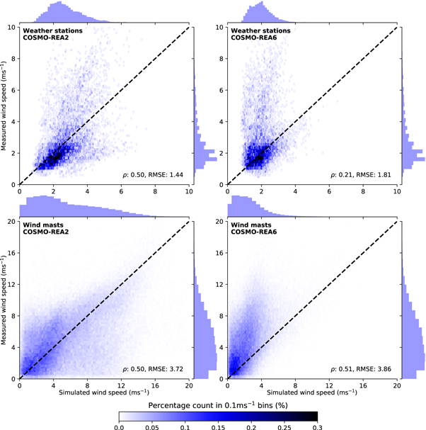
Figure 2. Heatmap comparison of simulated and measured wind speed according to anemometers at weather stations (top) and wind masts/turbines (bottom). Comparison is made for data in the period 2007–2013 with both COSMO-REA2 (left) and COSMO-REA6 (right) simulated wind speeds, with the number of data points given in table S.1. Weather station anemometers are situated 10 m above surface and record data at a monthly resolution. Wind mast and wind turbine anemometers are at heights above surface which vary between 40 and 100 m and record data at an hourly resolution. In all cases, simulation data are compared at the height of each anemometer. Dashed lines denote the ideal correlation between simulated and measured data; the deviation between simulated and measured data are given by the aggregated Pearson correlation (ρ) and root-mean-square error (RMSE), in the bottom-right of each subplot. ρ and RMSE at individual wind mast sites is given in table S.3.
Download figure:
Standard image High-resolution imageCOSMO-REA6 also under-predicts hourly measured hub-height data, but with a greater overall correlation than with weather station measurements (figure 2(b)). Since crests are smoothed out by the REA6 grid cell size, higher wind speeds are lost; very few wind speeds above 5 m s−1 are simulated (this can be seen across Switzerland in figure S.3). Performance as a function of height above surface cannot be readily compared, since the spatial and temporal distribution of the measurement sites are sufficiently different.
The relative performance of the COSMO reanalyses depends on the location (see table S.3). At four sites, COSMO-REA2 correlates best with measured data; at two other sites, COSMO-REA6 has a better correlation coefficient. The performance of both reanalyses is particularly poor at Gotthard, a narrow mountain pass, with a noticeable over- and under-prediction by COSMO-REA2 and COSMO-REA6, respectively.
3.2. Wind farm electricity generation
The COSMO reanalysis wind speed over- and under-prediction at wind sites leads to over- and under-predicted wind electricity generation, respectively. Figure 3 compares the performance of simulations based on COSMO-REA2 and REA6 with MERRA-2.
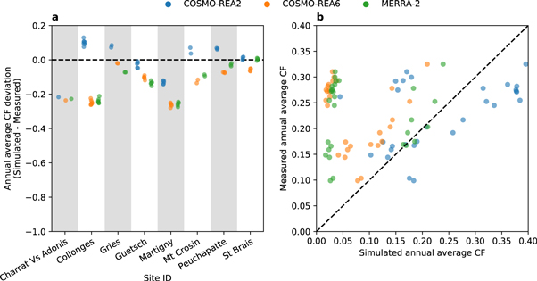
Figure 3. Performance of wind electricity generation simulations compared to measured annual wind farm data, for simulations derived from the VWF model using COSMO-REA2, COSMO-REA6 and MERRA-2 reanalyses. (a) The deviation in capacity factor at each site in each year in which there is available simulated and measured data. (b) Simulated against measured annual capacity factor for all sites and across all years in which there is available simulated and measured data. Markers in both subplots are coloured by the reanalyses from which wind speeds have been used in the VWF model. Simulations are undertaken at an hourly resolution, then averaged over each year. Only data points for the years 2007–2013 (the extent of COSMO-REA2) have been considered. For more information on each site, see table S.1. Dashed lines denote the ideal values for marker positions (no difference between simulated and measured data); the deviation is quantified for each reanalysis (aggregated across all wind farm sites) in table S.4.
Download figure:
Standard image High-resolution imageCOSMO-REA2 frequently outperforms the other reanalyses, particularly at Collonges, Guetsch, Martigny, and Mt. Crosin. However, at Gries, COSMO-REA6 deviates less in annual capacity factor than COSMO-REA2, and at Peuchapatte and St Brais, it is MERRA-2 which outperforms all other reanalyses. Across all sites, COSMO-REA2 is the best dataset to predict wind electricity generation; it has a lower RMSE and higher ρ than the other reanalyses (see table S.4). In fact COSMO-REA6 has a negative correlation between measured and simulated annual electricity generation.
The comparative advantage of COSMO-REA2 is also pronounced when considering hourly data. Figure 4 shows the load duration curve (LDC) of the turbine sites. The LDC orders the hourly capacity factor across the entire time series from greatest to smallest, then compares all datasets on a consistent x-axis of one year, irrespective of the length of each time series. Thus the x-axis of each dataset is multiplied by the ratio  . This allows us to assess the hourly variability of the data independently of exactly when in a year the variability occurs.
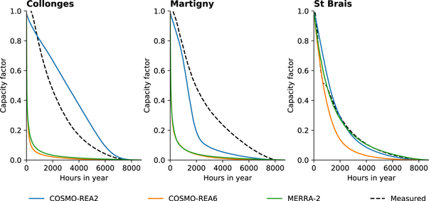
Figure 4. Load duration curve (LDC) of three Swiss wind farms, based on measured and simulated data. The LDC orders, from high (1) to low (0), the hourly capacity factor at a site across the entire time series. An LDC allows us to assess the hourly variability of the data independently of exactly when in a year the variability occurs. Both measured and simulation data are restricted to hourly data in the period 2007–2013 (the extent of COSMO-REA2), and only in hours for which there is measured data. Although several years are represented in the LDCs, traces have all been scaled to a single year (8760 h) on the x-axis; thus the x-axis of each trace is multiplied by the ratio  . Martigny and Collonges are valley sites, in the Rhone valley, while St Brais is a crest site in the Jura mountains; for more information on each site, see table S.1.
Download figure:
Standard image High-resolution imageIn the two Rhone valley sites (Martigny and Collonges), there is considerable under-prediction of the shape of the LDC. Although COSMO-REA2 does not match the measured LDCs, in these valleys it does fit better to the measured capacity factor than the other reanalyses (see table S.5). The significant under-performance of wind farms predicted by COSMO-REA6 and MERRA-2 at the two valley sites can be explained by their inability to resolve mountain-valley breezes. At St Brais, all reanalyses perform relatively well in reproducing the measured LDC, which can be attributed to the less complex terrain at the site's location in the Jura mountain range.
Summer diurnal variation in wind speed, and consequently electricity generation, is evident in the measured data shown in figure 5. The pronounced diurnal variation is captured by COSMO-REA2, albeit with a slightly different peak time and magnitude. However, COSMO-REA6 and MERRA-2 completely miss this; they predict that the summer electricity generation at these valley sites will not increase much above 20% capacity factor at any time during the day, whereas the measured data shows between a third and a half of hours are above 20% capacity factor at each site. The increased overnight wind speeds in summer at St Brais in the Jura mountain range is also captured by COSMO-REA2, and to a certain extent by MERRA-2, but only an afternoon peak is shown at this site in COSMO-REA6. In the winter, COSMO-REA2 correctly reproduces the variation in wind electricity generation on the Jura crests. However, it under-predicts output in Martigny and over-predicts in Collonges. This can also be seen in the LDCs given in figure 4. The systematic under-prediction of electricity generation at the valley sites of Collonges and Martigny is evident in the COSMO-REA6 and MERRA-2 results. At St Brais, as also seen with the annual data, the uncorrected MERRA-2 reanalysis outperforms all others in reproducing the LDC, followed closely by COSMO-REA2. Overall, we can conclude that none of the reanalyses reproduce reported electricity generation accurately in complex terrain, but generally, COSMO-REA2 outperforms the other reanalyses.
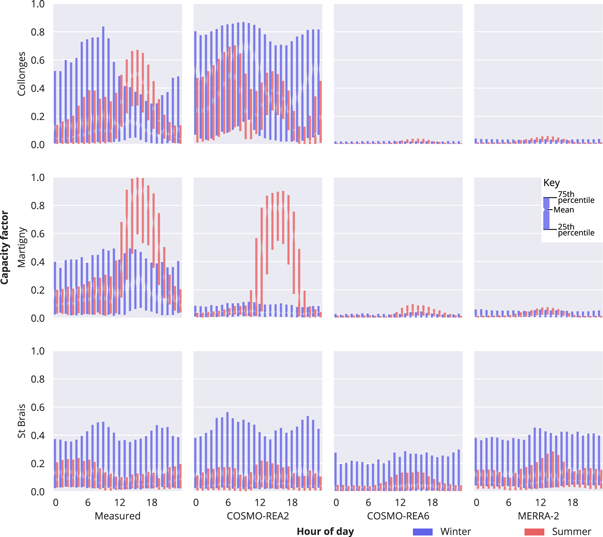
Figure 5. Seasonal diurnal variation at three wind farm sites in Switzerland, based on measured and simulated data. Each bar shows the interquartile range of capacity factor in a given hour, based on all days in each season, with a notch at the average (mean) capacity factor. The interquartile range is the subset of hourly data within the 25th and 75th percentile of the distribution describing the full dataset. Winter and Summer seasons cover the months of (December, January, February) and (June, July, August), respectively. Both measured and simulation data are restricted to hours in the winter and summer periods of 2007–2013 (the extent of COSMO-REA2), and only for hours in which there is measured data. Martigny and Collonges are valley sites, in the Rhone valley, while St Brais is a crest site in the Jura mountains; for more information on each site, see table S.1.
Download figure:
Standard image High-resolution image4. Spatio-temporal wind electricity generation variability
The complex terrain of Switzerland leads to meteorological phenomena which influence wind speed (see section S.1.3). On smaller scales, these are mountain-valley breezes due to terrain forcing and thermal forcing (Jafari et al 2012). On intermediate scales, these are channelling flows like the Föhn or Bise, caused by the alpine and Jura mountain ranges (Federal Office for Meteorology and Climatology 2015). On larger scales, these are the subseasonal weather regimes described in section 2.2. Given the demonstrated performance of COSMO-REA2 in capturing the mountain-valley breezes, we expect that it can also capture the impact of Bise and Föhn flows and weather regimes. Accordingly, we concentrate the remainder of this study on analysing spatio-temporal wind variability in selected regions of Switzerland. We select fourteen regions of interest in Switzerland that we expect to be impacted by mountain-valley breezes, Bise flows, Föhn flows, or the separation of weather systems on either side of the Alps (figure 6(a)). Details on these regions and the selection process are available in section S.1.4.

Figure 6. Characteristics of selected Swiss subregions. (a) Geographic extent of each subregion, using COSMO-REA2 grid cells, with orography given by line weight and opacity of each COSMO-REA2 grid cell. (b) Pearson cross correlation of hourly capacity factor in each region, for all hours in the period 2007–2013. Marker size and colour indicate degree of correlation. Correlation data for subregions studied further in section 4.1 are highlighted with a grey background. See section S.1.4 for more detail on selection criteria.
Download figure:
Standard image High-resolution imageThe complex terrain in Switzerland leads to a wide variation in wind conditions. Higher altitude regions (Alpine Crests, Gottard Pass, Jura Crests) have the highest mean capacity factor in winter, but three further regions have greater capacity factor than the Swiss average: Vedeggio Valley, Rhone Valley Knee, and Lake Geneva (figure 7). These regions might benefit from flow channelling. In the case of Vedeggio Valley and Rhone Valley Knee, this may be caused by strong inversion, in which cold air laying in either the lowlands or valleys might cause channelled density currents in the valley floor. Figure 8 inset 1 shows that blocking regimes (AR and EuBL) are the most performant regimes along the northern shore of lake Geneva, unlike the rest of Switzerland. The channelled Bise flow would be expected to be strengthened in both of these regimes.

Figure 7. Average seasonal capacity factor (CF) and diurnal standard deviation of CF in selected Swiss subregions, alongside the average Swiss CF in the same time periods, from both COSMO-REA2 and COSMO-REA6. Diurnal CF standard deviation is the standard deviation of CF across the average CF of all hours in the day, where the average CF is calculated for all days in a season. Diurnal CF standard deviation is an indicator of the strength of mountain-valley breezes in a region. See figure 6 for more detail on subregion characteristics and section S.1.4 for more detail on subregion selection criteria.
Download figure:
Standard image High-resolution image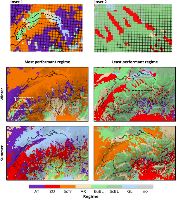
Figure 8. Seasonal most and least performant regimes in each COSMO-REA2 grid cell in Switzerland, and some parts of neighbouring countries. The highest performance regime in any grid cell is that with the greatest average capacity factor, calculated across all hours in a season classified by that regime (and vice-versa for the lowest performance regime). Switzerland is outlined in black. Orography is represented by grid cell outline (a darker outline signifies a higher altitude). Inset 1 shows the high performance of the blocking regimes AR and EuBL around Lake Geneva (highlighted with a dashed line), caused by the strength of the Bise flow in these regimes, which channels flow between the Northern Alps and the Jura range. Inset 2 highlights the ability of COSMO-REA2 to handle the complex terrain of Switzerland. The impact of ridges north of Zurich on suppressing wind speeds in the ZO regime in winter is clearly visible: with westerly ZO flow, low lying cold air dams ahead of the hills and hinders mixing. Winter and Summer seasons cover the months of (December, January, February) and (June, July, August), respectively.
Download figure:
Standard image High-resolution imageDiurnal variation in summer has a particularly strong impact in Upper Rhine Valley, Rhone Valley Knee, and Vedeggio Valley, as seen in figure 7. The strength of diurnal flows lead to a positive correlation between Upper Rhine Valley and Rhone Valley Knee, although they are on opposite ends of the country. Figure 6(b) shows that regions with similar dominant meteorological phenomena positively correlate, even when they are geographically separated. There is also a positive correlation between northern alpine valley outlets (Rhine Valley Outlet, Reuss Valley, Linth Valley, Linth Plain, Rhone Valley Outlet) and crests (Alpine Crests, Gottard Pass, Jura Crests).
South of the Alps, Vedeggio Valley and Magadino Plain correlate well. Hourly capacity factor in these two regions also correlate poorly with all other regions in the country. The meteorological divide created by the Alps is also evident in figure 8. In summer, the most and least performant regimes are inverted in the south compared to the north of the Alps. In winter, while not a direct inversion, different regimes are still more, or less, dominant in the two parts of the country.
To emphasise the ability of COSMO-REA2 to handle the complex terrain in Switzerland, inset 2 in figure 8 shows the impact of ridge lines north of Zurich on capacity factor. To the west of these five ridge lines there are small areas in which there is very low capacity factor in the ZO regime. This is an expected impact of elevated areas in otherwise flat, and low lying, terrain in the ZO regime: with westerly ZO flow, low lying cold air dams ahead of the hills and hinders mixing. Thus, near surface flow is decoupled from the stronger westerly flow which is apparent above the inversion. The same effect can be seen to the south of the Jura mountain range.
4.1. The role of Swiss wind power in Europe
Figure 9 compares seven of our selected Swiss regions with country-level aggregated data for Switzerland and its neighbouring countries (see section S.1.4.1 for the region selection). A more detailed comparison of intra-regime variability of the same selected Swiss subregions can be found in section 2.2. Compared to the Swiss average output, Lake Geneva shows a clear anticorrelation with all neighbouring countries in the AR and EuBL regimes. Similarly, Rhone Valley Knee shows anticorrelation with neighbouring countries in the ScBL and GL regimes.

Figure 9. Average hourly capacity factor during specific weather regimes in select subregions of Switzerland, compared to that of neighbouring countries. The average seasonal capacity factor in each subregion or country is given by grey bars, while the regime-specific capacity factors are given as deviations from this average. Neighbouring country data are taken from Renewables.ninja and are based on simulations using 'long term-future' wind farm deployment predictions and the MERRA-2 global reanalysis. Swiss nationally aggregated data are simulated both with MERRA-2 (via Renewables.ninja and 'long term-future' wind farm deployment predictions) and with a VWF simulation using COSMO-REA2 wind speed data. Swiss subregion data are based on a VWF simulation using COSMO-REA2 wind speed data. Winter and Summer seasons cover the months of (December, January, February) and (June, July, August), respectively, over the years 2007–2013.
Download figure:
Standard image High-resolution imageIn summer, Switzerland is particularly strong in the ZO regime, which anticorrelates with all neighbours except France. This performance is driven by the Upper Rhine Valley, Lake Geneva, and Rhone Valley Knee regions. South of the Alps, Vedeggio Valley matches Italy in its relatively high ScTr performance, but also does well in the AR regime and when there is no discernible regime. Although Jura Crests has a relatively high average capacity factor for Switzerland, its performant regimes generally match French and, to a lesser extent, German performant regimes. Hence, there is less of a capability for Jura Crests wind farms to capitalise on variations in the European electricity market. Yet, Jura Crests is the region with highest mean capacity factor, thus wind farms in the region are financially viable in their own right, and may even play a role in balancing wind generated electricity within the Swiss transmission system.
5. Discussion and conclusions
We used high-resolution regional reanalyses to investigate wind electricity generation variability in complex terrain with a focus on mountain-valley breezes, orographic channelling, and large-scale variability imposed by weather regimes. The relative performance of the reanalyses agree with that found by Jafari et al (2012), who showed that a 3 km grid was able to capture some of the complexity of the terrain, while a 9 km grid was no better than 25 km. Here, we see that a 2 km grid resolves some aspects of the complex terrain in Switzerland, but a 6 km grid is only marginally better than a ∼55 km grid. Thus there is a clear trade-off between geographic coverage and timespan on the one hand and spatial detail on the other. The short timespan and limited region covered by COSMO-REA2 is the price to pay for higher local detail, while the long timespan and global coverage of MERRA-2 comes with comparatively less local detail. COSMO-REA6 emerges with no clear advantage, however: its spatial resolution does not appear to give it a better performance than MERRA-2 over complex terrain, yet it covers a substantially shorter spatial extent and timespan.
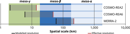
The poor performance of COSMO-REA6 and MERRA-2 could be explained by subdivisions of the mesoscale weather systems (figure 10) (Orlanski 1975). Both COSMO reanalyses are resolved at the meso-γ scale (2–20 km). However, only COSMO-REA2 has an effective resolution which could also capture meso-γ scale phenomena (14 km) (Wahl et al 2016). Indeed we see evidence that meso-γ scale phenomena are reproduced by COSMO-REA2 in the complex terrain of Switzerland. Meanwhile the effective resolution of COSMO-REA6 (48 km) lets it resolve meso-β scale phenomena (20–200 km) at best, and the effective resolution of MERRA-2 is likely to be around 200–400 km, i.e. within the meso-α scale.
Figure 10. Comparison of reanalysis resolution to scale of mesoscale weather system subdivisions. Grey areas refer to the difference between modelled and effective resolutions. MERRA-2 effective resolution is based on the working assumption in meteorology that effective resolution is normally 2–4 times higher than the model resolution.
Download figure:
Standard image High-resolution image
With COSMO-REA2, we are able to resolve the strong diurnal wind speed variation in valleys over summer (figure 5). While the magnitude of this variation differs between valleys, hourly profiles tend to correlate across northern alpine valleys (figure 6(b)). The northern alpine valleys anti-correlate with regions south of the Alps, which suggests that Föhn flow is also reproduced by COSMO-REA2. Finally, the Bise flow is resolved by the strength of wind speeds across lake Geneva during blocking weather regimes (figure 8). Based on these results, we find that electricity generation from wind turbines in specific regions of Switzerland should anti-correlate with those in the flat terrain of neighbouring countries. This result is particularly interesting because it cannot be seen when modelling Switzerland with models operating at coarser resolution, including COSMO-REA6 and MERRA-2.
At the very least, the patterns of anti-correlation we see should aid in balancing wind electricity generation and other variable renewable generation within Switzerland and similar countries. Whether they can also help smooth wind electricity generation within Europe is less clear, since most of the Swiss regions of meteorological interest are necessarily small, given they are located in mountainous terrain. The maximum technically feasible wind turbine capacity across all our selected Swiss subregions is 8.2 GW (based on land use data and a wind turbine power density of 8 MW km−2 (Tröndle et al 2019)), which is considerably less than the already existing capacity in neighbouring France, Italy, and Germany (Komusanac et al 2019). This would correspond to at most an annual generation of 18.2 TWh, or 30% of 2018 Swiss electricity consumption (Swiss Federal Office of Energy 2019). Less than 10% of this technical potential is likely exploitable in practice, since it does not even consider restrictions such as protected areas (Tröndle et al 2019). Nevertheless, these patterns may provide the economic incentive to kick-start wind turbine deployment in locations where average capacity factors would initially suggest unfavourable conditions. By relying on anti-correlation with other, and potentially much larger, wind-producing areas, wind farms in such locations could be economically attractive. This incentive is likely to be strengthened as wind turbine deployment continues to increase in the flatlands of Northern Europe. Moreover, diurnal variations could place Swiss wind farms in a favourable position during summer afternoon peak demand periods. However, this may compete with the current export of run-of-the-river electricity generation, which peaks in summer afternoons (Singh et al 2014). In addition, future electricity market design and the availability of economically attractive large-scale storage will influence the extent to which this exploitation of local wind patterns leads to economically attractive wind farm deployment.
Despite the new detail in local wind patterns revealed by COSMO-REA2, we have not studied smaller scale wind variability, which may not captured by COSMO-REA2 at all. Improved reanalysis products are still necessary, either by running models at higher resolutions, reaching 1 km or below, or by efforts to improve the effective resolution of existing reanalyses. In addition, we have seen that at specific sites in Switzerland, hourly measured wind speeds and electricity generation are not accurately reproduced by any of the reanalyses we investigate. It may also be possible to improve the accuracy of COSMO-REA2 by accounting for systematic bias in the reanalysis, in a similar manner to the MERRA-2 bias corrections performed by Staffell and Pfenninger (2016). However, the site-specific under- or over-prediction of capacity factor with COSMO-REA2 means that applying a national bias correction is unlikely to be possible and a spatially resolved bias correction would necessitate many more measurement sites across Switzerland.
Nevertheless, we did find that COSMO-REA2 captures the overall patterns of wind variability caused by key meteorological phenomena, which coarser spatial resolution reanalyses are unable to discern at all. These results are promising for energy modellers concentrating on complex terrain. To assess the contribution of wind power in such terrain to the energy system, accurately reproducing specific historical events may not be important as reproducing the patterns of variability at different time scales, such as anti-correlation with neighbouring sites, clear diurnal patterns, or specific behaviour in specific weather regimes. Understanding and exploiting these patterns of variability are ultimately what will influence the design and operation of reliable and cost-effective energy systems relying on large shares of variable renewable generation. Thus, existing studies comparing measured wind speeds with reanalysis wind speeds are perhaps not as relevant for energy modellers. Instead, reanalysis validation for energy modelling should undertake first to understand the meteorology of the regions of interest, then to identify the consistency of phenomena which are captured by simulations. A stronger focus on these phenomena may also open up new focus areas on which further development of meteorological reanalysis products for renewable energy applications should concentrate.
Acknowledgments
This study and the work of BP and SP was funded by the Swiss Federal Office for Energy (SFOE) under grant SI/501768-01. The contribution of CMG was supported by the German Helmholtz Association grant VH-NG-1243.
Data availability
The data required to simulate wind electricity generation were accessed from publicly available sources: Renewables.ninja and COSMO reanalyses. Some of the measured data that support simulation validation (section 3) are available in either aggregated or anonymised form from the corresponding author upon reasonable request. These data are not publicly available for legal reasons.