

Abstract
To improve air quality, China has been increasing the stringency of national emission standards for industrial sectors. However, from the projected air quality and associated health impacts it is not known if the updated emission limits have been completely followed. Here, we develop emission inventories based on the emission limits at different stages and use the Weather Research and Forecasting with Chemistry (WRF-Chem) model and health impact function to determine the potential air quality and health impacts for different scenarios. We found that full implementation of the special emission standards would decrease PM2.5 concentrations by over 25% in April, July and October, and decrease O3 concentrations in July by 10%–20%. Overall, the number of PM2.5-related premature deaths could be reduced by 0.15 million (95% confidence level 0.13–0.17 million) if special emission limits were met and that O3-related premature deaths would decrease by 18oo (95% confidence level 500–3000). However, even with these special emission limits, a greater than 25% increase in O3 levels occurred in northern China during October, January and April, leading to an increase in O3-related premature deaths in northern provinces which would offset the decrease in provincial PM2.5-related mortality by 10%–20%. These findings indicate that emissions of volatile organic compounds (VOCs) should be reduced to avoid increases in O3 in VOC-limited provinces. Despite the increase in O3 in certain provinces, improvement of industrial emission standards could greatly limit PM2.5 pollution and reduce the associated health burden. Therefore, we suggest that government should accelerate full implementation of strict emission standards in order to improve air quality.
Export citation and abstract BibTeX RIS

Original content from this work may be used under the terms of the Creative Commons Attribution 3.0 licence. Any further distribution of this work must maintain attribution to the author(s) and the title of the work, journal citation and DOI.
1. Introduction
In the past decade China has experienced serious air pollution problems. The degradation of air quality is characterized by high concentrations of fine particulate matter (PM) with aerodynamic diameters less than 2.5 μm (PM2.5) and surface ozone (O3). In 2017, PM2.5 was the major air pollutant (compared with PM10, O3, sulfur dioxide, nitrogen dioxide and carbon monoxide) on approximately three-quarters of all serious pollution days (Ministry of Ecology and Environment 2018), and the 90th percentile of the daily 8 h average O3 exceeded the air quality standard in approximately half of the 74 major cities in the summer (China National Environmental Monitoring Centre 2017). Long-term exposure to PM2.5 and O3 is closely linked to detrimental chronic health effects (Jerrett et al 2009, Burnett et al 2014), and short-term exposure is also associated with respiratory morbidity and mortality (Shang et al 2013, Bell et al 2014). It is estimated that PM2.5 could lead to approximately 1–1.5 million premature deaths in China annually (Hu et al 2017, Peng et al 2017, Song et al 2017) and that O3 pollution could cause 0.12–0.31 million premature respiratory-related deaths (Malley et al 2017).
The increase in PM2.5 pollution in China is attributed to the substantial anthropogenic emissions of primary PM2.5 and its precursors, such as sulfur dioxide (SO2), nitrogen oxide (NOx ≡NO + NO2) and volatile organic compounds (VOCs) (Huang et al 2014). Among the anthropogenic sources, industrial sources accounted for 87% of SO2 emissions, 69% of NOx emissions, 60% of primary PM2.5 emissions and 36% of VOC emissions in 2011 (Zheng et al 2018). The lack of stringent emission standards was one of the major reasons for these large quantities of industrial emissions. Before 2011, sector-specific emission standards were only established for thermal power plants, industrial boilers, the cement industry and the coke industry. Other industrial sectors followed a general standard for industrial kilns and furnaces, which allowed factories to emit large quantities of air pollutants (Ministry of Environmental Protection 1996). To reduce SO2, NOx and primary PM2.5 emissions from various industries, China accelerated the process of establishing and improving emission standards for the industrial sector (State Council 2013). These newly established standards allow industrial sectors to follow temporal emission limits for a few years and then transition to more stringent emission limits. These new emission standards, along with other pollution control measures in the industrial sector, contributed to reductions in SO2, NOx and primary PM2.5 emissions of 64%, 23% and 26% from 2011 to 2017, respectively (Zheng et al 2018). As a result, an annual reduction in PM2.5-related premature death of 0.25 million was achieved from 2013–2017 due to emission control (Ding et al 2019).
However, it is still unknown by how much PM2.5 emissions and the associated health burden could be reduced if the industrial sector were to completely conform to the emission standards for SO2, NOx and primary PM2.5. To evaluate air quality improvements, previous research used emission inventories that estimated emissions based on real data. The Multi-resolution Emission Inventory for China (MEIC; http://www.meicmodel.org/) (Zhang et al 2009, Li et al 2014, Zheng et al 2014, Liu et al 2015) calculated the real emissions of air pollutants using unpublished data from the Ministry of Environmental Protection to supplement the penetration rates of different emission control technologies (Zheng et al 2018). The Greenhouse Gas–Air Pollution Interactions and Synergies (GAINS) model (Amann et al 2011) developed an emission inventory for China considering the delay to legislation, as discussed by Zhao et al (2013) and Wang et al (2014). These studies all identified the industrial sector as a major contributor to future emission reduction, but very few have evaluated the relevant air quality and health impacts under an ideal scenario in which all the industrial sectors completely implement the new emission standards.
The impact of the updated emission standards on O3 pollution has also been largely ignored, and industrial VOC emissions have increased by 14% since 2011. Ground-level O3 is produced by photochemical oxidation of VOCs in the presence of NOx. This chemical process is a complex non-linear reaction. The sensitivity of O3 to NOx and VOC emissions depends on whether O3 production is NOx-limited or VOC-limited. In the NOx-limited regime, reduction of NOx emissions reduces the primary source of free oxygen atoms (NO2 photolysis) which react with O2 to form O3 (Milford et al 1989). In contrast, in a VOC-limited regime, NOx acts to reduce O3 (Kleinman 1994). Therefore, a decrease in NOx emissions would increase O3 concentrations under VOC-limited conditions (Jin and Holloway 2015). Additionally, a decrease in PM2.5 could slow the aerosol sink of hydroperoxy (HO2) radicals and thus stimulate O3 production (Li et al 2019). In 2017, the annual average O3 concentrations in the Beijing–Tianjin–Hebei region, Yangtze River Delta (YRD, Zhejiang, Shanghai and Jiangsu) and Pearl River Delta increased by 12%, 6.9% and 9.3%, respectively, compared with the concentrations in 2016 (Ministry of Ecology and Environment 2018).
In this research, we estimate the air quality and potential health impacts under the assumption that the published emission standards are fully implemented in industrial sectors. Using the emission inventories developed based on the emission standards of industrial sectors in four scenarios, we simulate air quality using the Weather Research and Forecasting with Chemistry (WRF-Chem) model and estimate the health impacts using an integrated exposure–response (IER) function.
2. Materials and methods
2.1. Descriptions of emission standards and scenarios
The sectors in our research include all the industrial sectors that are discussed in the Handbook of Industrial Pollution Sources (Ministry of Environmental Protection 2011). Specifically, the power sector is also considered as an industrial sector in this study. Detailed information on each sector is given in table S1 which is available online at stacks.iop.org/ERL/14/124058/mmedia. We designed four emission standards based on specific emission targets which are stated in the emission standards (table 1). All the emission standards can be found at http://kjs.mee.gov.cn/hjbhbz/bzwb/dqhjbh/dqgdwrywrwpfbz/. The Old Emission Standard assumes that all industrial sectors follow the emission standards published before 2004. Under the Old Emission Standard, sector-specific emissions standards were established only for cement, coke, boiler and electricity sectors, and all the other sectors follow the emission limits established in 1996. Moreover, in the Old Emission Standard, there were no emission limits for NOx emissions except for the nitric, cement and electricity sectors. In the updated emission standards that were established after 2004, there are two stages for the implementation of the new emission limits. The Temporal Emission Standard assumes that all industrial sectors follow the emission limits required in the first stage of the updated emission standards. In the Temporal Emission Standard, sector-specific emissions standards are established for most of the industrial sectors. Emission limits for smoke and dust are reduced by more than a factor in ferrous melting, non-ferrous melting and non-metal product sectors, and SO2 emission standards are greatly improved in the ferrous melting and coke industry. More importantly, specific emission standards for NOx are established. The New Emission Standard assumes that all industrial sectors follow the emission limits in the second stage, which are more stringent than those in the first stage. Compared with the Temporal Emission Standard, emission limits for SO2 are reduced by half or more in most sectors, while smoke, dust and NOx emission limits are reduced by about 40%. The Special Emission Standard assumes that all industrial sectors across China follow the lowest emission limits; this strategy was initially proposed for the North China Plain (NCP; Beijing, Tianjin, Hebei, Shanxi, Henan and Shandong). With the Special Emission Standard, nearly all the emission limits under the New Emission Standard are to be halved or more. In particular, the smoke emission limits for non-ferrous melting under the Special Emission Standard is one-eighth of that under the New Emission Standard. The emission limits for the implementation of the emission standards are shown in tables S2–S5. In this study, we calculated the quantities of SO2, NOx and primary PM2.5 emissions when the emission standards are completely implemented by industrial sectors and assumed that other air pollutants (including VOCs) remain unchanged.
Table 1. Descriptions of the four Emission Standards.
| Emission Standard | Description |
|---|---|
| Old | Established before 2004, mostly implemented by 2012 |
| Temporal | Established after 2004, mostly implemented between 2012 and 2015 |
| New | Established after 2004, mostly implemented after 2015 |
| Special | Established after 2004, implemented in seriously polluted areas |
According to the classification of the emission standards, we designed three scenarios. The Old → Temporal scenario assumes that the emission standards were updated from the Old to the Temporal standards. The Temporal → New scenario assumes that the standards are improved from the Temporal to the New standards. The New → Special scenario assumes that the New Emission Standard was changed to reflect the Special Emission Standard.
2.2. The compilation of the emission inventories
We used equations (1)–(4) to calculate provincial SO2, NOx and primary PM2.5 emissions in 2016 under different emission limits in the four emission standards. We did not calculate VOC emissions because only a few emission standards focused on VOCs, and VOC emissions from the industrial sector have continued to rise since 2010.


where i represents the industrial process (or fuel consumption of industrial boilers and power plants), k is the type of air pollutant, p is the province in China and q is the emission standard scenario.  represents the abated emission factor for product i following the emission limit of air pollutant k in scenario
  (m3 t–1) is the volume of smoke emitted from industrial process i.
  is the concentration limit (kg m–3) of air pollutant k in scenario q for the smoke emitted from process
  is the unabated emission factor for air pollutant k of process i.
  is the activity rate of industrial process i in province p.
  is the total emissions of air pollutant k from process i in province p.
  represents the total emissions of air pollutant k in province p.
  represents the industrial emissions of air pollutant k in MEIC grid r within the boundary of province p.
  represents the industrial emissions of air pollutant k in province p.
  represents the emissions of air pollutant k in grid r within the boundary of province p in scenario q. To avoid the influence of activity rates on emissions, we assumed that the production and fuel consumption in the industrial sectors remained the same as those in the year 2016.
The emission standards only regulate the emission limits for total suspended particulates (TSPs); therefore, equations (5)–(8) were developed to estimate the PM2.5, black carbon (BC) and organic carbon (OC) emissions.


where m is the available removal devices for PM, j is the type of removal device used to remove PM in scenario q,  is the rate of removal of TSPs during industrial process i under scenario q,
  represents the rate of removal of TSPs for device m during process i,
  is the rate of operation of PM removal device j during industrial process i in scenario q and approaches
  is the rate of removal of PM2.5 for device j during process i,
  represents the mass ratio of PM2.5 to TSPs during the industrial process of product i, and
  is the BC/OC mass ratio in PM2.5.
The concentration limits for SO2, NOx and TSP were based on the emission standards published from 1996 to 2016 (http://kjs.mee.gov.cn/hjbhbz/bzwb/dqhjbh/dqgdwrywrwpfbz/). The unabated emission factors and the volume of smoke were adopted from the Handbook of Industrial Pollution Sources (Ministry of Environmental Protection 2011). We collected provincial activity rates for industrial processes and fuel consumption in 2016 from the China Industrial Yearbook and China Energy Yearbook, respectively. The rates of removal of TSP and PM2.5 as well as the mass ratios of PM2.5, BC and OC were compiled from GAINS (Lei et al 2011, Klimont et al 2017). The rate of operation was based on the value used in the Asia-Pacific Integrated Model (Hibino et al 2003), and the modification of the emission inventory followed the method proposed by Peng et al (2017) and Qin et al (2017). The MEIC inventory (http://meicmodel.org) for 2016 was used to determine the spatial allocation of air pollutants. A validation and uncertainty analysis of the estimation is presented in table S7.
2.3. Configuration of the WRF-Chem model
WRF-Chem is a meteorological model coupled to a chemical mechanism that enables the simulation of atmospheric phenomena across scales ranging from meters to thousands of kilometers (Grell et al 2005, Fast et al 2006). In this study, we conducted simulations covering East Asia at a 30 km × 30 km horizontal resolution and with 36 vertical layers. The Carbon Bond Mechanism version Z (CBMZ) (Zaveri and Peters 1999) and Model for Simulating Aerosol Interactions and Chemistry (MOSAIC) (Zaveri et al 2008) were used to simulate the gas phase and aerosol chemical mechanisms, respectively. The initial conditions for meteorological variables were obtained from the Global Forecast System (GFS) of the National Center for Environmental Prediction (NCEP) analyses that are updated every 6 h. The chemical boundary and initial conditions were based on the archived simulations of the Model for Ozone and Related chemical Tracers (MOZART; www.acom.ucar.edu/wrf-chem/mozart.shtml) model. To improve the simulation of secondary inorganic aerosols, a new heterogeneous reaction was added to the CBMZ–MOSAIC chemical mechanism following the approach of Chen et al (2016) and Li et al (2017). The emission inventory developed for the four emission scenarios was based on anthropogenic emissions. The rest of the information describing the WRF-Chem model (e.g. the photolysis scheme) is presented in table S8.
Due to the high computational demands of these simulations, we simulated January, April, July, and October in 2016 as representative months for each season, with 1 week at the end of December, March, June and September used for model spin-up. In each season, the meteorological condition is different for the formation of PM2.5 and O3. Additionally, the contribution of industrial emissions to total emissions also varies with season. Therefore, we used the representative month of each season to reflect the seasonal change of meteorological conditions and emissions. The differences in air quality impacts due to different emission scenarios were evaluated by computing the changes in air pollutants.
We compared the monthly average of PM2.5 in our results with the 2016 PM2.5 observations (measurement stations are shown in figure S1, obtained from China National Environmental Monitoring Centre, http://106.37.208.233:20035/), and also compared the monthly average of the simulated daily maximum 1 h O3 with the 2016 O3 observations in figure S2. The normalized mean bias (NMB) and normalized mean error (NME) were used to evaluate the performance of simulation, which summarizes the discrepancy between the observation and the simulation. Figure S2 shows that NMB ranged between 0.1 and 0.4 for PM2.5 and 0.3 and 0.6 for O3, while NME was around 0.5 for PM2.5 and 0.7 for O3, which reasonably reproduce the observed PM2.5 and O3 concentrations fields compared with other research (Gao et al 2015, Chen et al 2016). Although there are underestimations at certain areas in some months, our model reasonably captured the general trend of observation. We also ran present-day simulations using 2016 MEIC data, and compared these with our simulations using the Temporal Emission Standard and New Emission Standard. We found that the temporal and spatial characteristics of PM2.5 and O3 in our results shared a pattern with those of the present-day simulations (figures S5 and S6).
2.4. Assessment of health impacts
We estimated the cause-specific premature deaths in each WRF-Chem grid using the relevant attributable fractions (Ezzati et al 2003), as recommended by GBD (GBD 2016 Risk Factors Collaborators 2017) and Environment Protection Agency (Cohan et al 2007):


where  is the number of premature deaths due to PM2.5 pollution or O3 pollution,
  is the baseline mortality rate for the exposed population, AF is the attributable fraction, RR represents the relative risk of death due to a change in the air pollutant concentration and
  is the exposed population in grid r (adults ≥ 25 years old).
We calculated the cause-specific premature mortality values attributed to long-term PM2.5 exposure following the IER function developed by Burnett et al (2014):
where z is the annual average PM2.5 concentration and  is the counterfactual concentration below which we assume that there is no health risk attributed to PM2.5. For PM2.5, we estimated the age-specific RR for mortality due to ischemic heart disease (IHD), stroke, chronic obstructive pulmonary disease (COPD) and lung cancer (LC). The values of parameters α, γ, δ and
  were given by the Global Burden of Disease Collaborative Network (2013).
The premature deaths due to long-term exposure to O3 were estimated following the method given by Silva et al (2016), where the daily maximum 1 h O3 concentrations is used in the health impact function:


where X is the average daily maximum 1 h O3 concentration,  is the change in O3 pollution and LCC (low-concentration cutoff) represents the threshold exposure concentration below which we assume there is no effect of O3 exposure on mortality. β is the concentration–response factor, which reflects the percentage change in mortality due to a unitary change in O3. According to Jerrett et al (2009), RR = 1.040 for a 10 ppb increase in the O3 concentration, and the average daily maximum 1 h O3 concentration was calculated in the consecutive 6 month period with the highest average. The value of LCC, derived from Malley et al (2017), is 33.3 ppb. In our research, the 2 months with the highest averages among January, April, July and October were used to estimate the average daily maximum 1 h O3 concentration. Additionally, we estimated premature deaths due to all chronic respiratory diseases.
We used the 30'' × 30'' global population distribution of the Center for International Earth Science Information Network (CIESIN), Columbia University (2016) from 2015 and regridded the population data to the WRF-Chem resolution (30 km × 30 km). The distribution of age groups was obtained from the 2010 Population Census of China. The baseline mortality rates for IHD, stroke, COPD, LC and all chronic respiratory diseases were collected from the Global Burden of Disease 2016 report (GBD 2016; http://ghdx.healthdata.org/gbd-results-tool).
To analyze the uncertainties associated with the RRs, baseline mortality rates and function parameters, we conducted 1000 Monte Carlo simulations. We assumed that the RRs of O3 follow a normal distribution with 95% confidential intervals (CIs), as reported by Jerrett et al (2009) and the GBD. For PM2.5, the parameter values used for the 1000 simulations were reported by the Global Burden of Disease Collaborative Network (2013). For baseline mortality rates, we assumed lognormal distributions with 95% CIs, as adopted from GBD 2016. The 95% CIs of the provincial mortality rates are shown in tables S9 and S10. The uncertainty ranges of the mortality shown in this study all refer to the uncertainty caused by the scientific uncertainty of the health function, and do not incorporate uncertainty from emissions or the air quality modeling.
3. Results
3.1. Emission reductions in different scenarios
Figure 1 shows the reductions in emissions under different scenarios. In total, SO2, NOx and PM2.5 emissions in the Old scenario would be reduced by 83.6%, 65.5% and 83.8% with the Special Emission Standards, respectively (table S7). The Temporal → New scenario contributed to the largest reduction in SO2 (7.6 Tg). Of the 7.6 Tg SO2 reduction, 45.8% was associated with the power sector, followed by the contributions of industrial boilers (23.5%) and the ferrous metal sector (16.0%). The Old → Temporal and New → Special scenarios both reduced SO2 emissions by approximately 4.5 Tg. The ferrous metal sector, industrial boilers and non-metal sectors contributed nearly 80% of the 4.3 Tg SO2 emission reduction in the Old → Temporal scenario, and the power sector accounted for over half of the emission reduction in the New → Special scenario.
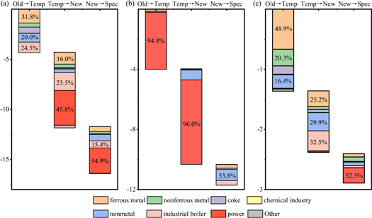
Figure 1. Emission reductions (in Tg) of (a) SO2, (b) NOx and (c) primary PM2.5 in the three scenarios and the contributions of industrial sectors to the emission reductions. Old → Temp represents the Old → Temporal scenario, Temp → New represents the Temporal → New scenario, and New → Spec represents the New → Special scenario.
Download figure:
Standard image High-resolution imageFor NOx emissions, the power sector accounted for 96.0% of the 5.9 Tg reduction in the Temporal → New scenario, and the power sector dominated the reduction in NOx emissions in the Old → Temporal scenario. In contrast, for the New → Special scenario, the reduction in NOx emissions in the power sector contributed little to this emission reduction, and the non-metal product sector accounted for over half of this reduction.
Shifting from the Old Standard to the Temporal Standard (Old → Temporal scenario) resulted in the largest reduction in most primary PM2.5 emissions (1.4 Tg), followed by those for the Temporal → New (1.0 Tg) and New → Spec (0.5 Tg) shifts. The ferrous and non-ferrous metal sectors contributed to 70% of the 1.4 Tg primary PM2.5 emission reduction in the Old → Temporal scenario. In the Temporal → New scenario, the improved emission limits for the industrial boiler, non-metal product and ferrous metal sectors accounted for nearly 90% of the reduction. For the New → Special scenario, the power sector accounted for approximately half of the reduced emissions.
3.2. Changes in air quality from the improving emission standards
Assuming that the emission standards are updated from the Old to the Special cases, figure 2 shows that the grid-level monthly average PM2.5 would decrease by 20 μg m−3 in eastern China and by less than 5 μg m−3 in western China (the geographical distribution of provinces is shown in figure S3). The largest percentage decrease in PM2.5 occurred in July, as more than 35% of the PM2.5 was reduced in eastern China, with peaks of more than 50% in northeastern (Inner Mongolia, Heilongjiang and Jilin; the distribution of provinces can be seen in figure S3) and southern (Jiangsu, Zhejiang, Jiangxi, Fujian and Guangdong) China. The smallest reduction in PM2.5 in eastern China occurred in January, when the monthly average PM2.5 was reduced by 10%–20% in northern China and by 20%–35% in southern China. Specifically, the NCP region experienced the most serious PM2.5 pollution (figure S5), and the monthly average PM2.5 was reduced by over 60–100 μg m−3 (35%–50%) in July, 40–80 μg m−3 (25%–35%) in April, 20–60 μg m−3 (20%–35%) in October and 10–40 μg m−3 (10%–15%) in January.
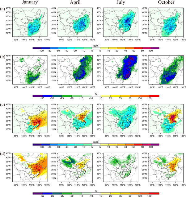
Figure 2. Changes after shifting from the Old Emission Standard to the Special Emission Standard: (a) change in monthly average PM2.5 concentrations, (b) percentage change in monthly average PM2.5 concentrations, (c) change in monthly average of daily maximum 1 h O3 concentrations and (d) percentage change in monthly average of daily maximum 1 h O3 concentrations during January, April, July and October.
Download figure:
Standard image High-resolution imageThe improvements in the emission standards also led to an increase in O3 pollution. Except in July, the monthly average of daily maximum 1 h O3 concentrations generally increased by over 20 μg m−3 in northern China. In January, most areas in eastern China experienced increases of over 50% in O3. In April and October, the O3 concentration generally increased by 25%–50% in northern China and decreased by 0%–15% in southern China. In contrast, the O3 concentrations decreased across China in July. Specifically, O3 decreased by 0%–10% in mid China, and other areas commonly observed decreases of 10%–20%.
Figures S7 and S8 show the changes in PM2.5 and O3 in each of the emission reduction scenarios. The Temporal → New scenario would result in the largest reduction in PM2.5, followed by the Old → Temporal and New → Special scenarios. In the Temporal → New scenario, a reduction of over 40 μg m−3 PM2.5 was achieved in the NCP region in July, with reductions of 20–30 μg m−3 in April, 10–20 μg m−3 in October and 2–10 μg m−3 in January. In the Old → Temp scenario, the reduction in PM2.5 was approximately 10 μg m−3 less than that in the Temp → New scenario, except in the NCP region. In January, PM2.5 in the NCP decreased by 10–20 μg m−3 in January in the Old → Temp scenario and decreased by 2–10 μg m−3 in the Temporal → New scenario.
The largest increase and decrease in O3 both occurred in the Temporal → New scenario. In the Temporal → New scenario, the increase in surface O3 exceeded 40 μg m−3 in the NCP in October and YRD in January and October. The largest decrease in O3 occurred in July in the Temporal → New scenario, as O3 decreased by 10–20 μg m−3 in the NCP and 20–30 μg m−3 in the YRD and southern China. In the Old → Temporal scenario, the increase in O3 occurred over a more widespread area. In July in the Old → Temporal scenario, O3 increased by 2–20 μg m−3 in Jiangsu, Anhui, Shandong, Henan, Tianjin and Hebei, and the O3 concentrations in these provinces generally decreased in the Temporal → New scenario. Furthermore, in April, the increase in O3 covered larger areas of the NCP and YRD in the Old → Temporal scenario than that in the Temporal → New scenario. Additionally, in January in the Old → Temporal scenario, O3 increased in the southern provinces (e.g. Fujian, Sichuan and Yunnan), which was not the case in the Temporal → New scenario. For the New → Special scenario, the increase in O3 was less than or equal to 10 μg m−3 in January and April and less than or equal to 20 μg m−3 in October. In particular, in April, Anhui and Jiangsu provinces exhibited decreasing O3 concentrations in the New → Special scenario, and O3 increased in these provinces in the Old → Temporal and Temporal → New scenarios.
3.3. Health impacts related to updated emission standards
Figure 3(a) shows the change in the number of annual premature deaths due to PM2.5 and O3 in the 30 provinces in China (except Tibet and Taiwan) after shifting from the Old Emission Standard to the Special Emission Standard. For the PM2.5-related premature deaths, eastern, central and southern China generally experienced higher reductions in mortality than other geographical regions. The largest reduction in PM2.5-related premature deaths occurred in Guangdong [15.2 × 10³, 95% CI (12.5–17.7) × 103], followed by Jiangsu, Shandong, Hebei and Henan (over 104 in each province). Considering the population, the highest decrease in premature deaths per capita occurred in Shanghai (143 per million population, 95% CI 125–162), followed by Guangdong and Jiangsu (figure S9(a)). In total, by improving the emission limits from the Old Standard to the Special Standard, the 1.4 × 10⁶ [95% CI (1.1–1.6) × 106] PM2.5-related premature deaths under the Old Standard could be reduced by 0.15 × 10⁶ [95% CI (0.13–0.17) × 106]. Due to the nonlinearity of the health assessment model, the health burden was only reduced by 10.9%, although PM2.5 concentrations were reduced by more than 25% in most areas.

Figure 3. (a) The changes in the annual number premature deaths due to PM2.5 and O3 in the 30 provinces of China (except Tibet and Taiwan) after shifting from the Old Emission Standard to the Special Emission Standard and (b) the initial air pollution-related premature deaths following the Old Emission Standard in 30 provinces and the provincial reduction of annual air pollution-related premature deaths if the Special Emission Standard is fully implemented. The two dashed lines represent that the ratio of PM2.5-related premature deaths to O3-related premature deaths and equal 5:1 and 10:1, respectively. The geographic classification of the provinces can be found in table S9. The number of air pollution-related premature deaths is the sum of the PM2.5-related premature deaths and O3-related premature deaths.
Download figure:
Standard image High-resolution image
The changes in premature deaths related to O3 varied by geographical region in China. VOC-limited regimes were found in northern and eastern provinces, while most southern provinces were NOx-limited (Jin and Holloway 2015). This geographical difference means that reducing NOx emissions would increase O3 concentrations in northern and eastern provinces and decrease O3 concentrations in southern provinces. As a result, the O3-related premature deaths in northern China and eastern China generally increased, with a maximum change in Hebei Province (1100, 95% CI 500–1500). However, after considering the effect of population, Beijing and Tianjin experienced the largest increase in O3-related premature deaths per million population. The increase in O3 partly reduced the health benefits due to the decrease in PM2.5 in several provinces. The increase in premature deaths due to O3 offset approximately 20% of the decrease in PM2.5-related premature deaths in Beijing and Tianjin and 10% of those deaths in Hebei and Shandong. In contrast, deaths due to O3 decreased in southern China and southwestern China. The largest reduction in O3-related premature deaths (1000, 95% CI 400–1400) occurred in Sichuan Province. Following Sichuan Province were Jiangxi and Hunan, which experienced reductions of 990 (95% CI 400–1300) and 930 (95% CI 380–1300) O3-related premature deaths. As for the reduction in premature death per capita, the largest decrease occurred in Jiangxi and Guangxi provinces. Based on the total change in premature deaths in all provinces, the premature deaths attributed to O3 decreased by 1800 (95% CI 500–3000) after shifting from the Old Emission Standard to the Special Emission Standard.
Figures S12 and S13 show that the changes in premature deaths due to O3 are strongly related to the reduction scenario. Specifically, O3-related premature deaths increased by 3200 (95% CI 1400–4200) in the Old → Temporal scenario, and the largest increases occurred in Shandong (820), Jiangsu (790), Henan (540) and Hebei (530). Conversely, O3-related premature deaths decreased by 2400 (95% CI 920–3500) and 2700 (95% CI 1100–3700) in the Temporal → New and New → Special scenarios, respectively. The changes in PM2.5-related premature deaths are consistent with the changes in PM2.5 concentrations (figure S10). Premature deaths attributed to PM2.5 decreased the most in the Temporal → New scenario [69.8 × 10³, 95% CI (60.7–78.3) × 103], followed by the changes in the Old → Temporal [45.9 × 10³, 95% CI (40.4–51.2) × 103] and the New → Special scenarios [29.3 × 10³, 95% CI (29.3–38.3) × 103].
Figure 3(b) shows the total change in premature deaths (by combining the change in PM2.5-related and O3-related premature deaths) and the initial premature deaths (by combining PM2.5-related and O3-related premature deaths) in the Old Emission Standard. There is a strong linearity between the total reduction in premature deaths and the initial premature deaths. Larger health benefits commonly occurred in provinces with a larger number of initial premature deaths. Figure S9(b) reveals there is less linearity between the total reduction of premature deaths per capita and the initial premature deaths per capita. Northern and central provinces generally experienced higher initial premature deaths per capita, but larger reductions per capita occurred in southern and eastern China.
4. Discussion
In this study, the air quality and health impacts were estimated assuming that various emission standards were fully implemented. We observed a large reduction in PM2.5 if the emission standards are improved to the most stringent stage, with a peak of over 50% in summer. Specifically, in southern China, complete implementation of the Special Emission Standard could result in a large decrease in air pollution of 35% or more. However, during wintertime, assuming emission limits are improved to the most stringent standard, PM2.5 in the NCP would be reduced by only 10%–15%, and this percentage reduction in PM2.5 was far from the target value (25%) set by the government. Additionally, in northern and eastern China, the decrease in PM2.5 was accompanied by a sharp increase in O3 during spring, autumn and winter. By improving the industrial emission standards, we estimated that up to 0.15 × 10⁶ [95% CI (0.13–0.17) × 106] PM2.5-related premature deaths could be avoided each year. Additionally, 1800 (95% CI 500–3000) O3-related premature deaths could be avoided. However, O3-related premature deaths increased in northern provinces and offset 10%–20% of the health benefits associated with the decreased PM2.5 concentrations.
Our results indicate that there would be a significant if the industrial factories completely conform to the new industrial emission standards. Currently, factories are forced to reduce production or even shut down during wintertime. These measures contribute much to the improvement of air quality, but also slow down economic growth. If the emission standards were fully implemented, the reduction measures could be less aggressive. Improving the emission standards could also stimulate factories to adopt cleaner technology. To reach the increasingly stringent emission limits, more factories would upgrade their production structure. Natural gas may be more widely used to provide power and heat in industrial sectors, which generates much less air pollution than coal.
However, it is challenging for the Chinese government to ensure that each plant is fully implementing the emission standards. The power sector is the most promising to achieve full implementation of the Special Emission Standard. The Chinese government has been focusing on reducing emissions from coal-fired plants since 2005, and much advanced equipment have already been installed. For the other sectors, there are more barriers to complete conformity to even the Temporal Emission Standard. As there were no specific emission standards for most industrial sectors before 2012, many sectors have not installed end-of-pipe devices. To meet the Temporal Emission Standard between 2012 and 2015, and then sharply improve to the New Emission Standard in 2016, substantial investment is required to equip and upgrade the devices over a short period. This aggressive improvement would increase the financial burden on small factories. Generally, the Old and the Temporal Emission Standards are more likely to be fully implemented, as current devices to remove air pollutants could easily reach the emission limits. In contrast, it is difficult to achieve full implementation of the New and Special Emission Standards because the required removal efficiency of the air pollutants nearly meets or exceeds the maximum efficiency of the available end-of-pipe devices. The introduction of new end-of-pipe devices with better performance would require much more investment, and therefore producers are generally not motivated to apply these new pollution control measures. The central government has established inspection teams to determine whether plants have followed emission standards and other regulations. However, the inspection teams cannot supervise all plants at all times. To continuously supervise the plants, China has installed a Continuous Emissions Monitoring System (CESM) at the largest plants, which reports real-time emissions data to the government. Although the CESM has improved the efficiency of data collection, Karplus et al (2018) noted that the CESM data do not correspond to the satellite observations, implying falsification of the CESM data. In addition to improving the supervision system, other measures could be used to improve the implementation of the emission standards. An environmental tax would force the plants to introduce end-of-pipe devices with high removal efficiencies to avoid penalties. Another option is to allow more time for emitters to comply with tougher standards but with strict enforcement. If plants are found to falsify data or violate the standards, higher penalties should be imposed. For example, the government could shut down those plants that fail to follow the standard or report falsified data.
Although the finding suggests that air quality could be greatly improved if the updated emission standards were fully implemented in industrial sectors, other sources of air pollutants should also be controlled to further improve air quality. Specifically, the agriculture sector is the major source of ammonia (NH3) emissions, and NH3 is an important precursor of secondary PM2.5. Additionally, the residential sector is the major source of primary PM2.5 in northern China during the winter. The implementation of emissions standards would also increase the health risk due to O3 pollution, particularly in the NCP and YRD regions. To avoid an increase in O3-related deaths in these VOC-limited provinces, the emission of VOCs should be mitigated along with NOx emissions. As over half of the VOC emissions are sourced from vehicles and solvent use, more stringent emission standards for the transportation sector and solvent use should be established.
5. Caveats
Several limitations need to be overcome in any future research. Firstly, we assumed that the volume of smoke (V in equation (1)) followed the Handbook of Industrial Pollution Sources (Ministry of Environmental Protection 2011). However, the volume of smoke varies greatly in the real world (table S6). Therefore, this assumption would lead to uncertainties in our estimation (table S7). Another uncertainty in our approach is the estimation of primary PM2.5 emissions. The emission standard only states emission limits on TSPs not on primary PM2.5, BC or OC. We used the operation rates and removal rates of end-of-pipe devices to estimate primary PM2.5 emissions and used the mass ratio of BC and OC in PM2.5 to estimate PM2.5, BC and OC emissions. In table S7, we estimated the uncertainty range of our estimation, and compared our results with those of Zheng et al (2018), who estimated the real emissions in 2016. We found that the estimated 2016 SO2 emission from Zheng et al (2018) is higher than that under the New Emission Standard and lower than the Temporal Emission Standard, and the NOx emission was within the confidence interval under the Temporal Emission Standard.
Secondly, in the model configuration, our model underestimated PM2.5 and O3 concentrations in certain areas, which may lead to an underestimation of change in PM2.5 and O3. The bias between observed and simulated values is inevitable as it is rather challenging to fully reproduce the observed concentrations over China. Several factors led to the uncertainties in our simulation. Firstly, there are uncertainties in the emission inventory (Zhao et al 2011), including anthropogenic emissions, biogenic emissions and wildfire emissions. Secondly, there are uncertainties during the simulation of meteorological conditions (e.g. wind field, boundary conditions, cloud and precipitation), which would influence the simulation of air pollutants. Thirdly, there are also limitations in the chemical mechanism. One advantage of our simulation is that we have improved the chemical mechanism of sulfate and nitrate by incorporating heterogeneous reactions into the model. However, there is still underestimation of secondary inorganic aerosols during peak hours even though the heterogeneous mechanism was added to the model (Chen et al 2016). Additionally, recent studies on the heterogeneous mechanism mostly focus on improving the simulation in North China (Zheng et al 2015, Chen et al 2016, Li et al 2017), and therefore the simulation is more capable of capturing the PM2.5 field in the north than the south. Due to these limitations, our model could not fully capture the observed concentration fields, and this might influence our prediction of the health impacts.
Lastly, there are also large uncertainties in applying the IER function. We used country-level baseline mortality rates in the function, as provincial data for age-specific and cause-specific mortality rates are unavailable. Using different GBD datasets would lead to significantly different estimations due to differences in mortality rates, population distribution, counterfactual concentration and other parameters (Ostro et al 2018). As the data and methods are the most up to date, we used the datasets from GBD 2016 in our research. Additionally, we used 30 km × 30 km horizontal resolution in our research, as the finest horizontal resolution for the MEIC inventory available is 0.25°×0.25° and our research domain covers a large area (the whole of China). A coarse horizontal resolution is unable to reflect the realistic spatial concentration gradients, especially near the source region, due to averaging effects. Studies have found that a coarse horizontal resolution would under-predict the maximum concentrations while over-predicting minima (Arunachalam et al 2011). Nonetheless, previous studies indicated that the horizontal resolution has somewhat modest effects on premature deaths attributable to O3 as well as PM2.5 exposures. Punger and West (2013) calculated a less than 6% increase in O3-related premature deaths in the United States when using a 100–400 km resolution compared with a 12 km resolution. Thompson et al (2014) indicated that the difference in PM2.5-related health impacts when using different horizontal resolutions is within 10%. Besides, as the shape of the health impact function is concave, the impact of the uncertainties in PM2.5 and O3 on the change in premature deaths is also limited compared with the uncertainties in the health impact function (Liu et al 2016). Large-scale cohort studies of PM2.5 and mortality are absent in the most polluted countries, and the magnitude of the excess RR from PM2.5 exposure at high levels of PM2.5 remains uncertain in the IER function (Cohen et al 2017). Long-term exposure to the chemical components of PM2.5 has not been well studied (Lepeule et al 2012), and we used the total PM2.5 concentration to estimate premature deaths in the health impact function. The health impact model in our study has not considered indoor air pollution, which may underestimate health effects due to indoor coal combustion (Meng et al 2019). There is also less evidence for the relationship between O3 and COPD. However, a large body of literature has supported a causal link between increased COPD mortality and long-term exposure to O3 (Atkinson et al 2016). There is also uncertainty due to the use of the O3 metric in the health impact function. The daily maximum 1 h O3 and 8 h average of O3 are both commonly used to evaluate the health impacts of O3 (Turner et al 2016, GBD 2016 Risk Factors Collaborators 2017). In this research, the simulation of maximum 1 h O3 performed better than that of maximum 8 h O3 in capturing the O3 observation fields, and therefore we used the daily maximum 1 h O3 in the health impact function. The limitation of our approach is that we used the O3 over a 6 month period, which would overestimate the O3 concentration over mid-latitude areas where there is substantial annual variation of O3 (Monks et al 2015). Another limitation is that Jerrett et al (2009) derived the RR independent of PM2.5 from a multi-pollutant model, but within the model there was a moderate correlation between O3 and PM2.5 (Malley et al 2017).
Acknowledgments
This work was supported by funding from the National Key Research and Development Program of China (2016YFC0206202), the National Natural Science Foundation of China (under award nos 41571130010, 41671491, 41390240) and a Newton Advanced Fellowship (NAFR2180103). We also thank Xiaodong Zhang for the assistance.
Data availability statement
The data that support the findings of this study are available from the corresponding author upon reasonable request. The data are not publicly available for legal and/or ethical reasons.