

Abstract
A growing literature documents the effects of heat stress on premature mortality and other adverse health outcomes. Urban heat islands (UHI) can exacerbate these adverse impacts in cities by amplifying heat exposure during the day and inhibiting the body's ability to recover at night. Since the UHI intensity varies not only across, but also within cities, intra-city variation may lead to differential impact of urban heat stress on different demographic groups. To examine these differential impacts, we combine satellite observations with census data to evaluate the relationship between distributions of both UHI and income at the neighborhood scale for 25 cities around the world. We find that in most (72%) cases, poorer neighborhoods experience elevated heat exposure, an incidental consequence of the intra-city distribution of income in cities. This finding suggests that policymakers should consider designing city-specific UHI reduction strategies to mitigate its impacts on the most socioeconomically vulnerable populations who may be less equipped to adapt to environmental stressors. Since the strongest contributor of intra-urban UHI variability among the physical characteristics considered in this study is a neighborhood's vegetation density, increasing green space in lower income neighborhoods is one strategy urban policymakers can adopt to ameliorate some of UHI's inequitable burden on economically disadvantaged residents.
Export citation and abstract BibTeX RIS

Original content from this work may be used under the terms of the Creative Commons Attribution 3.0 licence. Any further distribution of this work must maintain attribution to the author(s) and the title of the work, journal citation and DOI.
1. Introduction
Replacement of natural land cover with built-up structures, coupled with dense human activity, increases the local temperature in cities compared to the background climate—a phenomenon known as the urban heat island (UHI) effect (Oke 1982). When combined with increasing global mean temperatures and heatwaves, the UHI effect exacerbates human health risk (Milan and Creutzig 2015, Tewari et al 2019). Since over two-thirds of the global population will reside in urban areas by 2050, heat stress in urban areas will impact a disproportionate fraction of us in the future (Gerland et al 2014).
Extreme heat can have pronounced and potentially dramatic public health implications, including heat stroke, dehydration, and exacerbation of existing medical conditions, like cardiovascular and cerebrovascular disease, diabetes, chronic obstructive pulmonary disease, pneumonia and asthma, and increased mortality (Tan et al 2010, Shahmohamadi et al 2011, Heaviside et al 2017). Heat waves also lead to physical and mental stress, as well as increased susceptibility to food and vector-borne infectious diseases (Shahmohamadi et al 2011).
The associated health impacts of the UHI effect can have differentiated impacts across populations. Certain urban residents, particularly those of lower socioeconomic status, with pre-existing health conditions, or living in dense urban areas, have been found to be exposed to higher levels of UHI and its negative health outcomes (Solecki et al 2005, Jenerette et al 2007). Case studies in China, Japan, the United States, and Europe suggest that socioeconomic vulnerability is associated with UHI exposure, extreme heat morbidity or mortality (Robine et al 2008, Wilhelmi and Hayden 2010, Gronlund 2014, Hsiang et al 2017, Nayak et al 2018).
Most studies on socioeconomic disparities in heat exposure are predominantly based on LST—a measure that is heavily influenced by geography, seasonality and background conditions (Lindley et al 2006)—and focuses on heat wave events at a regional scale without consideration of persistent heat exposure due to the UHI effect, except for individual cities (Solecki et al 2005, Jenerette et al 2007, Tomlinson et al 2011). In fact, most UHI studies have been conducted for limited case studies with a focus on wealthier cities in more developed contexts. Given the wide variety of measurement techniques used in existing UHI studies, comparing results between cities to understand what factors influence the distribution of UHI's impacts and how UHI mitigation interventions perform is challenging.
As an initial step towards filling this gap, we provide the first multi-city analysis of the association between surface UHI distribution and neighborhood-scale income data by combining satellite remote sensing with census data. Importantly, we consider a range of cities from different geographic regions and levels of economic development to see whether observed effects are widespread or unique to particular types of cities. This paper is organized as follows: section 2 elaborates the methodology used in this study, section 3 discusses the results and section 4 discusses the implications for policy and decision-making.
2. Methodology
2.1. Selected cities
We selected 25 cities from the Urban Environment and Social Inclusion Index (UESI; Hsu et al 2018) data set. These cities are located in climate zones and countries representing a variety of economic development levels and environmental circumstances. From the 32 cities in the UESI we chose only those for which neighborhood-scale income data are available. Consequently, they should not be considered a random sample (e.g. the cities selected may be more established compared to new or emerging cities), and our results should be interpreted with that caveat in mind. Nonetheless, this set of cities is useful both for illustrating the approach we developed to provide measures of inequalities in urban heat distribution within and between cities, and for providing an initial understanding of these equity impacts across the globe. Table S1 is available online at stacks.iop.org/ERL/14/105003/mmedia and provides descriptive statistics for each city.
2.2. Data processing
We process and extract the neighborhood-level satellite measurements using the Google Earth Engine platform (Gorelick et al 2017). Two categories of variables are generated for each neighborhood: (1) UHI intensity and (2) three factors or urban-rural differentials for the physical characteristics of cities that are associated with the UHI effect. For each city, the year of the satellite data extracted corresponds to the most recently available data for population and income (table S1). Neighborhoods smaller than the satellite product resolution (1 km × 1 km) are excluded, since no unique observations can be extracted for these.
The UHI intensity is defined as the area-averaged differential in land surface temperature (LST) between neighborhood i and a rural reference r as measured by the NASA AQUA satellite's moderate resolution imaging spectroradiometer (MODIS) sensor

The rural reference includes all non-urban land pixels within city boundaries, as classified in the European Space Agency Climate Change Initiative land cover data (Bontemps et al 2013). This methodology is an extension of the Simplified Urban Extent algorithm, previously used to estimate surface UHI intensity at a global scale (Chakraborty and Lee 2019). We only include pixels with an uncertainty of less than 3 °C (Wan and Dozier 1996). The average elevation of each city, as well as its rural reference are extracted from the GMTED product (Danielson and Gesch 2011) and shown in table S1.
We calculate proxies for three factors that modulate the UHI: vegetation density, degree of urbanization, and shortwave reflectivity (Peng et al 2011). Similar to UHI, we construct these variables for each neighborhood by calculating area-averaged differentials between each neighborhood and its city's rural reference. The normalized difference vegetation index (NDVI)—a standard index for greenness—reflects the fact that live green vegetation absorbs most of the radiation in the red band (which can be utilized for photosynthesis), and reflects most of the radiation in the near infrared (Rouse et al 1974).
The vegetation differential ΔNDVIi is given by:
Here, NIR and RED are the surface reflectances in the near infrared and red (bands 2 and 1) of the 500 m resolution MODIS Aqua Surface Reflectance 8-Day product (MYD09A1.006).
The normalized difference built-up index (NDBI) is a proxy for the degree of urbanization, capturing the fact that urban areas reflect more in the shortwave infrared band than in the near infrared (Zha et al 2003). The urban built-up differential ΔNDBIi is:
Here, SWIR is the surface reflectance in the shortwave infrared band (band 6) of MYD09A1.006. We use only the highest quality pixels, based on band-specific quality control flags that correct for, among other things, cloud contamination, high solar zenith angle, and detector noise.
The surface albedo is the reflectivity of a surface in the shortwave wavelength range, a critical factor controlling local temperature. The albedo differential Δαi is the difference in total reflectivity between a neighborhood and the rural reference. Total reflectivity is the weighted average between black sky albedo (BSA) and white sky albedo (WSA), where the weight k is the ratio of diffuse fraction of solar radiation for the pixel of interest (Qu et al 2015). For each neighborhood

We calculate k for the grid that houses a city's centroid using the 15-year mean (2003–2017) of the NCEP/NCAR reanalysis data (Kistler et al 2001). Observations of WSA and BSA are from the MODIS 16-Day Albedo product (MCD43A3.006) at 500 m resolution and are quality controlled to reduce cloud contamination. Singapore and Jakarta, however, experience significant cloud contamination, preventing data extraction for the reference pixels. For these cities, we include lower-quality and cloud-contaminated data.
While many others factors, like anthropogenic heat flux, longwave trapping by urban canyons, aerosols, etc can modulate the UHI (Taha 1997, Zhao et al 2014, Li et al 2018), two of the factors considered in this study account for the vast majority of UHI mitigation measures; green roofs and green spaces modulate NDVI, while white roofs and reflective pavements alter α (Rizwan et al 2008, Zhao et al 2017). The third factor, NDBI, is the UHI's most direct cause since it is a proxy for the degree of urbanization. The advantage of using urban-rural differentials instead of absolute values, e.g. ΔNDBI versus NDBI, is the recognition that these different cities are located in distinct background climate zones. Using these differentials standardizes the impacts of urbanization and imposes soft limits on what mitigation efforts cities can reasonably achieve through reducing any deviations from the unperturbed state of the land cover.
We merge the satellite-derived data with neighborhood-scale income and population data. The primary data sources vary by country, but are typically per capita household income or disposable income taken from cities' or countries' own census databases or surveys (Hsu et al 2018).
2.3. Evaluating equity of UHI distributions
We use techniques developed in the health and welfare economics literature to analyze equity of UHI distributions (Maguire and Sheriff 2011). Lorenz curves (Lorenz 1905) and concentration curves (Wagstaff et al 1991) provide graphical unit-free representations of distributional equity. Lorenz curves depict the cumulative percent of the variable of interest (income or UHI exposure) accruing to a cumulative population percentile ranked from worst to best off. Concentration curves show the cumulative UHI exposure accruing to a cumulative percentile of the population, ranked from poorest to richest. Due to the data resolution, our analysis abstracts from within-neighborhood variability, assuming that income and environmental variables are equally distributed within each neighborhood unit.
The closer a Lorenz or concentration curve is to a 45° line dividing the cumulative population and income or environmental concentration axes, the more equal a variable's distribution. A concentration curve lying above the 45° line would be pro-wealthy, while one below would be pro-poor. Since concentration curves require positive values of the environmental variables, we normalize UHI intensity and city physical characteristic values to have a minimum value of zero.
To facilitate cross-city analysis, we also calculate Gini coefficients and concentration indices, summary measures of the area between the 45° line and the Lorenz and concentration curves, respectively. The Gini coefficient ranges from zero to 1, with a higher value indicating a less equal distribution. The concentration index ranges from −1 to 1. For an undesirable outcome such as UHI, a negative value indicates a pro-wealthy distribution and a positive value indicates a pro-poor distribution. Both indices provide summary measures of intra-city inequality.
3. Results
3.1. Neighborhood-scale surface UHI intensity
The mean daytime UHI intensity varies quite widely between cities, from 7.19 °C for Mexico City to 0.36 °C for Johannesburg (figure 1), and shows similar magnitudes when 10-year mean values are used instead of the years corresponding to availability of census data (figure S1). The cities cover the Köppen–Geiger climate zones (Rubel and Kottek 2010) with the major human habitations (CIESIN 2012). The daytime UHI values are generally higher than the nighttime values (figures 1 and S3(d)), although they are not strongly correlated (figure S2) since they emerge due to different reasons—difference in evaporation, convection, and shortwave reflectively between urban and rural areas during the day and differential release of stored heat and anthropogenic heat flux at night, among other factors (Peng et al 2011, Zhao et al 2014, Chakraborty et al 2017).

Figure 1. Daytime surface UHI intensity of the cities considered. The mean UHI intensity of each city is given by the points, while the error bars represent the standard deviation across different neighborhoods of the city (i.e. variability of the UHI within cities). The color of the point represents the background climate zone the city is situated in and the gray vertical line is for a UHI value of 0 °C. The data are extracted for the same year as the available income data.
Download figure:
Standard image High-resolution imageIn estimating absolute UHI intensity, geographic units based on physical changes associated with urbanization are preferable to politically-defined administrative boundaries (Chakraborty and Lee 2019), since they more closely relate to the physical factors driving UHI. Intra-city census tracts, for which socioeconomic data are collected and available, however, are almost always based on administrative boundaries. We therefore apply an administratively-defined urban boundary with neighborhood-level divisions to examine intra-city variation and its association with neighborhood-scale income. This level of aggregation at the neighborhood scale using administrative definitions are also useful in decision-making and policy contexts because they may align with zoning and other planning instruments.
3.2. Neighborhood-scale income and UHI intensity
3.2.1. Income and UHI Inequality
The Lorenz curves show that UHI is not equally distributed within most cities. Figures S4 and S5 indicate that for only four cities in our sample—Atlanta, Barcelona, Johannesburg, and Sao Paulo—is daytime or nighttime UHI more equally distributed than income (the UHI Lorenz curve is closer to the 45° line). The Lorenz curves contain no information regarding how the UHI burden is allocated across income groups. The UHI intensity concentration curves in figure 2, however, reveal that about half the cities (Atlanta, Berlin, Buenos Aires, Copenhagen, Jakarta, Johannesburg, Los Angeles, Melbourne, Mexico City, Montreal, Tokyo, and Vancouver) have a noticeably pro-wealthy UHI intensity distribution, which means that the greater UHI burden falls on the poor. Of these, Berlin, Buenos Aires, Copenhagen, Jakarta, Los Angeles, and Vancouver's UHI concentration curves clearly show a disproportionate impact on the lowest income-earners. Eight cities (Atlanta, Amsterdam, Barcelona, Chicago, Detroit, New York, Seoul, and Singapore) lack an observable systematic UHI bias with respect to neighborhood income, while the remaining six cities (Beijing, Bangkok, London, Manila, Paris, and Sao Paulo) have a pro-poor distribution.

Figure 2. Environmental concentration (EC) curves of UHI (blue) and Lorenz curves (red) for each city in the study. An EC curve above the 45 equity line indicates that UHI intensity is more heavily allocated to the less affluent districts. If the EC curve is located below the 45 equity line, UHI is more intense in the wealthier areas of the city.
Download figure:
Standard image High-resolution image3.2.2. Typologies of UHI and income inequality
To summarize these results for cross-city comparison, in figure 3 we classify each city into one of four typologies (Hsu et al 2018) by comparing where cities fall with respect to four quadrants formed by the Concentration Index (x-axis) and Gini Index (y-axis). 44% of the cities of the sample are located in the top left quadrant (Quadrant 1), where inequality in UHI distribution is allocated to lower income districts: a 'pro-wealthy' condition—and could compound the existing, albeit relatively low, income inequality within each city. Lower-income residents in these cities might lack the capacity to cope with increased temperature associated with the UHI. 28% of the cities are located in the bottom left quadrant (Quadrant 3) where unequal UHI distribution compounds the relatively high income inequality. On the other hand, 20% of the cities are located in the top right quadrant (Quadrant 2), where UHI intensity is more heavily allocated to the wealthiest citizens, creating what could be call a 'pro-poor' situation, where increased UHI affects citizens that may be less vulnerable. Finally, 8% of the cities (London and Sao Paulo) are in the bottom right quadrant (Quadrant 4) where UHI inequality is affecting the more affluent citizens and there is relatively high income inequality. Among the cities, Johannesburg stands out due to having the highest income inequality in the sample, as well as a relatively high inequality of UHI intensity.

Figure 3. Four-quadrant plot of daytime UHI concentration and Gini indices for cities in the study. The quadrant threshold (i.e. x-intercept) for the concentration index is 0, while the y-intercept for the income Gini is the mean Gini of the sample cities (0.17). The size of the points represent the magnitude of daytime UHI intensity in degrees Celsius.
Download figure:
Standard image High-resolution image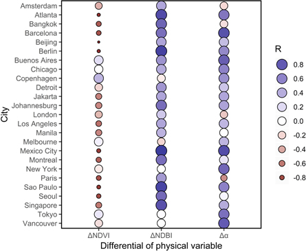
Figure 4. Correlation between neighborhood-scale daytime surface UHI and urban-rural physical characteristic differentials, namely Δα, ΔNDVI, and ΔNDBI. The values, represented by both color and size of the circles, reflect the Pearson correlation coefficient.
Download figure:
Standard image High-resolution image3.3. Physical characteristics of cities and their impact on UHI intensity
To identify implications of potential policy interventions for addressing inequities in the UHI distribution, we consider the distribution of ΔNDVI, ΔNDBI, and Δα for the cities. Cities usually have lower vegetation compared to rural areas due to replacement of vegetated land with built-up structures, which means NDVI and NDBI are inversely correlated (figure S6). Therefore, ΔNDVI is generally negative (figure S3(c)), meaning greenness and surface vegetation are reduced due to urbanization. We observed the highest difference between urban and rural land cover within the city for Paris and Barcelona and the lowest for Detroit and Singapore. Similarly, ΔNDBI shows positive values and is highest for Sao Paulo and lowest in Los Angeles. There is not a clear trend for Δα between cities since urban land cover can have a higher or lower α (Taha 1997). In general, white surfaces like concrete have a higher α than vegetation, meaning they reflect more sunlight; urban areas also have darker surfaces, like asphalt pavements, which reflect very little solar radiation. The relation between urban and rural α also depends on the background vegetation in the urban area, with darker vegetation being less reflective than lighter vegetation. Overall, these complexities lead to a mixed association between neighborhood-scale ΔNDVI and Δα (figure S7).
We examine the associations between neighborhood-scale daytime surface UHI and the Δα, ΔNDVI, and ΔNDBI for each city (figure 4). In general, we see a negative correlation between UHI and ΔNDVI, since more vegetated neighborhoods have higher evaporative cooling, and thus, lower surface temperatures, as demonstrated at various scales (Rizwan et al 2008, Peng et al 2011, Chakraborty et al 2017, Chakraborty and Lee 2019). A few cities, like Buenos Aires, Copenhagen, Melbourne, and Tokyo do show slight positive relationships between UHI and ΔNDVI. These are coastal cities, where the sea breeze front also modulates local temperature, and thus the UHI intensity (Hu and Xue 2016). All else equal, green space is replaced by built-up structures in urban areas. Thus, we observe a positive association between UHI and ΔNDBI. Finally, there is a positive correlation between daytime UHI and Δα, as also seen in Peng et al (2011), although this relationship is complicated due to individual city characteristics and the correlation between Δα and ΔNDVI. For instance, cities for which UHI is negatively correlated with Δα also have strong positive correlations between UHI and ΔNDVI (figure S7). Since the urban-rural differentials used here are the absolute values of the physical characteristics of a neighborhood offset by a constant rural reference, the associations would remain same even if the absolute values of the physical characteristics had been used instead.

Figure 5. Scatterplots for daytime UHI concentration index and ΔNDBI concentration index (a) and daytime UHI concentration index and ΔNDVI concentration index (b) for cities in the study. Pearson correlations (R), significance (p-values), and quadrant of cities are given for each plot.
Download figure:
Standard image High-resolution image
4. Discussion
This study provides the first quantitative analysis of the UHI effect's unequal distributional impacts at the neighborhood level across multiple cities. With the adoption of the 2030 United Nations Sustainable Development Goals 11 (SDG-11), there is broad recognition in global policy agendas for sustainable and inclusive urban growth that minimizes inequality (United Nations 2017). There are sparse data available, however, for urban policymakers to understand whether they are on track to achieving SDG-11 (Hsu et al 2018). By analyzing the UHI through the lens of distributional equity, we demonstrate that existing inequality is associated not only with a city's income distribution, but also with environmental stressors like urban heat. These hidden inequalities—where lower-income residents are exposed disproportionately to greater UHI—go unaccounted for in many scientific studies and policy considerations (Wilhelmi and Hayden 2010, Chan et al 2012, Gronlund 2014, Nayak et al 2018).
Despite some cities boasting strong environmental track records and performance (Hsu et al 2018), these results suggest that cities still have room to improve with respect to designing focused policy interventions that address distributional equity and alleviate environmental inequalities (EEA 2018, Nayak et al 2018). High per capita income cities with relatively equal income distributions and low absolute levels of UHI effects, such as Copenhagen, Berlin, or Vancouver, nonetheless have a UHI distribution that falls more heavily on the less affluent. On the contrary, many cities in developing countries have a UHI burden that is less 'pro-rich' although the absolute intensity of the effect is relatively high.
Our results also indicate that UHI exposure is associated with a city's development pattern (figures S3 and 5(b)) and the drivers that affect the spatial distribution of residents (Brueckner and Fansler 1983, Cullen and Levitt 1996, Marcińczak et al 2016). For instance, the highest levels of UHI distribution inequity are located in countries like Brazil, the United States, and South Africa—countries with high income segregation within cities (OECD 2018). Similarly, several aspects of urban development, such as housing market, connectivity to main commercial districts, and access to amenities affect whether more affluent citizens live in the city center—where UHI intensity is generally higher due to the physical mechanisms involved in its formation (i.e. higher degree of urbanization, lower vegetation cover, higher anthropogenic heat flux, more built-up structures with higher thermal mass, etc)—or in the suburbs where UHI is less intense (Glaeser et al 2008, OECD 2018). For instance, the majority of the cities with extreme urban heat exposure in poorer neighborhoods (UHI concentration index <−0.1), namely Buenos Aires, Vancouver, Copenhagen, and Los Angeles, are coastal cities, with higher income neighborhoods situated along the waterfront, leaving poorer residents in city centers where UHI intensities are highest. Clustering cities according to their location in the four-quadrant typology (figure S8) illustrates these patterns in cities' UHI versus income inequality distribution, shedding light on possible policy solutions that could be shared between cities in similar clusters.
To address the inequality of UHI distribution, cities have several mitigation options demonstrated through our analysis of greenness, built-up environment, and surface reflectance. As cities develop, they tend to reduce the availability of green space, which decreases evaporative cooling (Taha 1997)—a side-effect of urban growth. It is thus unsurprising that a pro-rich distribution of NDBI is associated with a pro-rich distribution of UHI (figure 5(a)). Assuming that urban vegetation is desirable, i.e. a negative concentration index value is pro-poor, figure 5(b) shows that cities with pro-poor UHI distributions tend to have pro-poor vegetation cover distributions (figure S9).
UHI mitigation strategies may need to be targeted at populations that have the greatest need due to their disproportionate exposure or low capacity to cope with the associated health effects. There is evidence that combining multiple UHI mitigation strategies can effectively negate the localized warming due to both UHI and climate change (Zhao et al 2017). In an increasingly urbanized future, intertwining different UHI mitigation strategies can potentially transform cities into havens of climate adaptation, since city-level policy making can bypass constraints often present at other government levels (Hoffmann 2011, Hsu et al 2015).
While the method presented in this paper is applicable to other environmental burdens or goods, there are limitations. Due to data availability, we are only able to collect income as a crude proxy of neighborhood-level socioeconomic status available for all cities in the sample, although a range of other factors (e.g. race and ethnicity) that result in inequality could also be used if available and context-appropriate. There may also be inconsistencies in definitions and data-collection methods for neighborhood-level income data between cities. Secondly, spatial mismatches between a remotely-sensed urban agglomeration and administrative boundaries inhibit comparable neighborhood definitions between cities. For instance, Tokyo and Bangkok's administrative boundaries only include its central districts, while Sao Paulo and Beijing have much broader boundaries that include rural neighborhoods that are sparsely populated. Given the objective of this paper and the data limitations, the administrative boundaries were used. However, with more granular socioeconomic data, a more consistent unit of analysis may be possible in future research.
Another limitation is our use of the Earth's surface temperature instead of air temperature to estimate the UHI, since air temperature is more strongly coupled with heat stress. Even though UHI at the surface and near-surface air can have different seasonal and diurnal trends (Chakraborty et al 2017), the use of satellite-derived LST is advantageous when studying multiple cities since most cities do not have high resolution measurements of air temperature. Monitoring this intra-urban variation in air temperature is necessary to better quantify the spatial distribution of urban heat and its consequences for urban dwellers. Finally, this initial analysis consists of a single snapshot in time. For policy-making, it is important to understand how relationships between characteristics like UHI intensity and income are shaped, both in terms of city-wide aspects such as development patterns, but also about individual behavioral responses. If people demonstrate a willingness to pay for lower heat exposure (Klaiber et al 2017), pro-poor investments in vegetation enhancements in poor neighborhoods may increase rents, potentially pricing out the intended beneficiaries.
5. Conclusion
Cities vary significantly in their exposure to the UHI and how the UHI is distributed across varying socioeconomic groups within their administrative boundaries. This spatial variability also extends to a city's physical characteristics. In almost all the cities considered, the presence of urban green vegetation in a neighborhood moderates the UHI's magnitude. In 72% of our sample cities, the UHI disproportionately affects residents of lower socioeconomic status, an issue that occurs for both developed and developing cities alike. A pathway forward for addressing the UHI should involve more careful consideration towards equalizing the benefits of UHI and climate mitigation strategies to spaces or citizens that are disproportionately affected. Including these strategies that consider differential and unequal impacts as a relevant element of urban development can prevent increased exposure as a negative externality of urban growth.
Data availability statement
All data produced in this article are available upon reasonable request.