


Abstract
The growing share of variable renewable energy increases the meteorological sensitivity of power systems. This study investigates if large-scale weather regimes capture the influence of meteorological variability on the European energy sector. For each weather regime, the associated changes to wintertime—mean and extreme—wind and solar power production, temperature-driven energy demand and energy shortfall (residual load) are explored. Days with a blocked circulation pattern, i.e. the 'Scandinavian Blocking' and 'North Atlantic Oscillation negative' regimes, on average have lower than normal renewable power production, higher than normal energy demand and therefore, higher than normal energy shortfall. These average effects hide large variability of energy parameters within each weather regime. Though the risk of extreme high energy shortfall events increases in the two blocked regimes (by a factor of 1.5 and 2.0, respectively), it is shown that such events occur in all regimes. Extreme high energy shortfall events are the result of rare circulation types and smaller-scale features, rather than extreme magnitudes of common large-scale circulation types. In fact, these events resemble each other more strongly than their respective weather regime mean pattern. For (sub-)seasonal forecasting applications weather regimes may be of use for the energy sector. At shorter lead times or for more detailed system analyses, their ineffectiveness at characterising extreme events limits their potential.
Export citation and abstract BibTeX RIS

Original content from this work may be used under the terms of the Creative Commons Attribution 3.0 licence. Any further distribution of this work must maintain attribution to the author(s) and the title of the work, journal citation and DOI.
1. Introduction
To mitigate future climate change an energy transition to low or zero-carbon energy sources is required (e.g. Matthews et al 2009, Meinshausen et al 2009). For this reason, in many places the share of renewable wind and solar power generation of total power generation is increasing. This growing share of variable renewable energy increases the sensitivity of power systems to meteorological conditions and their variability. Wind and solar electricity production, and also electricity demand all depend on the weather and therefore exhibit variability at hourly, daily, weekly, seasonal and annual timescales (e.g. Kavak Akpinar and Akpinar 2005, Pryor et al 2006, Sinden 2007, Suri et al 2007, Bessec and Fouquau 2008, Bloomfield et al 2016). It is paramount to consider the spatial and temporal variations in energy production and energy demand in the design and operation of future power systems with a high share of renewable sources (Armaroli and Balzani 2011, Zeyringer et al 2018).
To guarantee a continuous and secure energy supply in a future highly-renewable power system, critical situations require special attention. In Europe, large-scale high pressure systems can lead to the unfortunate combination of low wind and solar power production and high energy demand, resulting in extreme high energy shortfall (Bloomfield et al 2018, Van der Wiel et al 2019a). The flexibility requirements of a power system are, in part, determined by such events (Huber et al 2014). System adequacy analyses, e.g. the ability to meet peak demand, taking into account the full range of meteorological variability and power system characteristics are thus essential to identify, and design for, critical events (Armaroli and Balzani 2011).
To meet the societal need for information on the dependence of energy production and energy demand on weather and climate, an interdisciplinary scientific discipline is developing rapidly: 'energy meteorology'. The meteorological community has contributed with insights into the effects of interannual meteorological variability on energy production and demand (Klink 2002, Pryor et al 2006, Davy and Troccoli 2012, Haupt et al 2016, Kumler et al 2018), the influence of the North Atlantic Oscillation (NAO, e.g. Pozo-Vázquez et al 2004, Brayshaw et al 2011, Ely et al 2013, Jerez et al 2013, Curtis et al 2016, Zubiate et al 2017, Ravestein et al 2018), expected changes due to further climate change (Pryor and Barthelmie 2010, Hueging et al 2013, Jerez et al 2015b, Haupt et al 2016, Reyers et al 2016, Craig et al 2019), and the seasonal predictability of energy-related variables (Clark et al 2017, Thornton et al 2019). However, the relationship between meteorology, energy impacts, and critical events is complex and therefore needs tailored studies.
This study aims to investigate whether weather regimes adequately represent the influence of meteorological variations on the European energy sector. Weather regimes are classifications of common atmospheric circulation regimes (figure 1) and have proven to be useful in weather forecasting and climate change applications (e.g Reinhold 1987, Ferranti et al 2015, Neal et al 2016, Matsueda and Palmer 2018). They influence the weather at the surface (e.g. Trigo and DaCamara 2000, Plaut and Simonnet 2001, Yiou and Nogaj 2004, Santos et al 2005, Yiou et al 2008, Donat et al 2010), hence influencing renewable power generation and electricity demand (Grams et al 2017, Thornton et al 2017). Meteorological and energy forecasts are of value for the energy sector, that plans operations and resource adequacy, and trade on electricity markets based in part on this information (Pinson et al 2013). Specifically, this study answers two questions: (i) what are the average impacts of the weather regimes on energy variables? and (ii) are energy extremes linked to a specific weather regime? We quantify the day-to-day variability of energy variables and the risk of extreme or critical events in each weather regime. Our focus is on the winter season, in which the weather regimes (Sanchez-Gomez et al 2009, Lavaysse et al 2018) and the variability of total wind and solar energy production and demand (Van der Wiel et al 2019a, their figure 8) are most pronounced. We take a compound system approach, taking into account the combined effects of wind and solar power production, and energy demand.
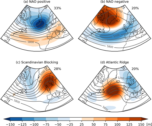
Figure 1. Four regimes of atmospheric circulation in the North Atlantic-European domain, (a) NAO positive, (b) NAO negative, (c) Scandinavian Blocking, (d) Atlantic Ridge. Colours show the 500 hPa height anomaly (m), contour lines show the 500 hPa height (m, interval 100 m) indicative of the direction of flow. The percentage values denote the percentage of total days categorised in each regime. Figure based on ERA5 data (DJF, 1979–2018).
Download figure:
Standard image High-resolution image2. Methods
2.1. Meteorological data
We used the ERA5 reanalysis product (Copernicus Climate Change Service 2017) to represent observed historical meteorological conditions (Olauson 2018, Urraca et al 2018, Ramon et al 2019). The full ERA5 record available at time of analysis was used, 1979–2018, providing 40 years of data. The analysis of variability, in particular for the occurrence of extreme events, is hindered by the limited length of the observed record (Bloomfield et al 2016, Van der Wiel et al 2019a). In the 40 year ERA5 record just four 1-in-10 year extreme events can be sampled. We therefore also used data from two large ensemble experiments created using two Global Climate Models (GCMs): EC-Earth (v2.3, Hazeleger et al 2012) and HadGEM2-ES (Martin et al 2011). Each large ensemble experiment contains 2000 years of simulated weather for present-day conditions. This allows an analysis of how 200 extreme events in each model dataset, with return periods of 10 years and longer, are distributed over the different weather regimes. Details on the large ensemble GCM experimental setup are provided in Van der Wiel et al (2019b) and Blackport and Screen (2019). The GCMs reproduce the observed temporal occurrence, surface impacts and variability of/within weather regimes (see supporting information, SI, which is available online at stacks.iop.org/ERL/14/094010/mmedia).
2.2. Weather regime classification
Each winter day (December, January, February (DJF)) in the ERA5 record was assigned to one of the four North Atlantic weather regimes (Vautard 1990, Michelangeli et al 1995) following the classification method of Cassou (2008). Clustering was done based on daily maps of anomalous 500 hPa geopotential height (units: m) in the North Atlantic-European region (90◦W-30◦E, 20◦-80◦N). The first fourteen Empirical Orthogonal Functions (EOFs) patterns were computed (Dawson 2016), which captured 89% of total variance. The associated Principle Component time series (PCs) were used as coordinates of a reduced phase space. K-means clustering was then used to compute four centroids, and to assign each daily map to a centroid. The K-means algorithm aims to separate the maps in groups of equal variance and minimises the within-cluster sum of squares (Pedregosa et al 2011).
The clustering of GCM data was done in a slightly modified manner. Instead of computing the EOF patterns from the simulated daily maps itself, the EOF patterns from ERA5 were used and fourteen pseudo-PCs were computed for each GCM. These pseudo-PCs were then used to assign each daily map to the centriods as determined from ERA5 data. As expected the spatial pattern of the resulting weather regimes is similar, the temporal occurrence of each regime was not constrained and shows agreement between ERA5 and the GCMs (SI figure S1). The modified method was applied to ensure maximum spatial similarity of the weather regimes between the ERA5 data and the GCM data. Physically this is relevant because slight differences in the location of high/low pressure systems in a regime can have larger impacts on the surface impacts, and can therefore influence the weather regime-to-energy relation of interest here.
2.3. Energy model
To link the weather regimes to impacts relevant for the energy sector, daily wind and solar power production and electricity demand were calculated. The energy model used to make these calculations is described here in brief; for the full model description including model equations we refer the reader to Van der Wiel et al (2019a).
Spatial patterns of daily wind and solar power potentials (units: %) were considered, a quantity that depends only on the meteorological state, not on installed wind turbine or solar cell capacity. Wind power potential was calculated using a power curve profile dependent on wind speeds (Jerez et al 2015a), a hub-height of, respectively, 80 and 120 m for onshore and offshore locations was assumed. Solar power potential was calculated using incoming solar radiation and a solar cell temperature-based performance metric which depended on temperature, incoming solar radiation and wind speed (TamizhMani et al 2003), solar panel tilt was neglected. For the calculation of total European power production (units: TWh d−1), a projected spatial distribution of installed capacity over fifteen western European countries7 was assumed (Van der Wiel et al 2019a).
Energy demand (units: TWh d−1) was computed using a regression model calibrated using historical demand data and a population-weighted European mean temperature value (Van der Wiel et al 2019a). The daily difference between energy demand and renewable wind and solar energy production is referred to as energy shortfall or residual load.
2.4. Analysis
For each of the weather regimes, the average meteorological surface and energy impacts were determined by means of composite analysis, i.e. the mean over all days classified in the regime. Anomalies—departures from normal conditions—were computed by subtracting a DJF-mean climatology. The length of the ERA5 record allowed us to robustly compute the composite mean patterns, the analysis and figures in the main manuscript are therefore based on ERA5 data. Equivalent figures for the GCM experiments served as a validation of the simulated data (SI figures S2, S3).
We further considered the variability of energy variables within each weather regime. To do so, a systematic comparison of the four regimes to each other and to the full sample, all winter days, was made. Since sampling issues are of concern here, we show both the ERA5 data and the GCM data in the main manuscript. We considered extreme events of at least a 10 year return period, it was assumed there are four such events in the 40 year ERA5 record and 200 events in each 2000 year GCM experiment. Estimates of change in the risk of occurrence of an extreme event were based on the risk ratio (or probability ratio), a metric commonly used in climate attribution studies:

with PWR the probability of an extreme event given a weather regime, and Pclim the probability of an extreme event in the full sample. RR = 1 indicates no change in risk, RR > 1 indicates increased risk of an extreme event occurring given that weather regime, RR < 1 indicates decreased risk given that weather regime. Risk ratios noted in the text are averages of the two GCMs.
3. Results
3.1. Weather regimes and average meteorological and energy impacts
Atmospheric circulation patterns for the four North Atlantic weather regimes are shown in figure 1. Two regimes resemble the positive and negative phase of the NAO (Hurrell et al 2003): the 'NAO positive' regime (figure 1(a), 33% of days), characterised by an anomalous low pressure system over Iceland and higher than normal pressure in a band to the south, and the 'NAO negative' regime (figure 1(b), 20% of days), with anomalous high pressure over Greenland/Iceland and lower than normal pressure to the south. A third regime, 'Scandinavian Blocking' (figure 1(c), 28% of days), is characterised by anomalous high pressure over Scandinavia and lower than normal pressure to the south and west. Finally, the fourth regime is distinguished by a positive pressure anomaly over the North Atlantic and a negative anomaly over Europe (figure 1(d), 20% of days), this regime is referred to as 'Atlantic Ridge'. These patterns match similar classifications in earlier research (e.g. Vautard 1990, Michelangeli et al 1995, Cassou 2008).
The anomalous position of pressure systems enhance or disturb the typical zonal, west-to-east, flow. Contour lines in figure 1 show the flow direction at 500 hPa height. Days classified as NAO positive typically have a stronger than normal zonal flow, in the other regimes the normal zonal flow is weakened over parts of the European continent.
For energy applications the impacts of the weather regimes at the surface are relevant. The flow at 500 hPa discussed above influences the progression of weather systems over the continent, and therewith influences surface variables such as the near-surface wind speed and temperature. Figure 2 shows the typical surface imprint of the four weather regimes on relevant meteorological variables, while figure 3 shows the effect on wind and solar power potentials. These anomalies of power potential only lead to changes in power production if wind turbines or solar cells are installed in the region of surface impacts. Sections 3.1.1–3.1.4 describe the mean spatial meteorological and energy characteristics of each regime.
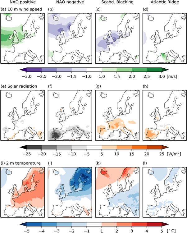
Figure 2. Mean meteorological surface impacts of the four weather regimes. Colours show anomalies of (a)–(d) 10 m wind speed (m s−1), (e)–(h) incoming solar radiation (W m−2), (i)–(l) 2 m air temperature (°C). Each weather regime in a column, labelled at the top, left to right: NAO positive, NAO negative, Scandinavian Blocking, Atlantic Ridge. Figure based on ERA5 data (DJF, 1979–2018).
Download figure:
Standard image High-resolution image
Figure 3. As figure 2 but here for mean power production impacts of the four weather regimes. Colours show anomalies of (a)–(d) wind power potential (%), (e)–(h) solar power potential (%). Each weather regime in a column, labelled at the top, left to right: NAO positive, NAO negative, Scandinavian Blocking, Atlantic Ridge. Figure based on ERA5 data (DJF, 1979–2018).
Download figure:
Standard image High-resolution image3.1.1. NAO positive
The enhanced zonal flow during NAO positive days leads to higher than normal 10 m winds over the North Sea, Denmark, Ireland, the Netherlands and the United Kingdom (figure 2(a)). Westerly winds from relatively warm ocean surfaces lead to higher than normal 2 m temperatures in central and northern Europe (figure 2(i)). Incoming solar radiation is close to normal for the time of year (figure 2(e)).
These conditions lead to higher than normal wind power potential in the North Sea area (figure 3(a)). Over the southern North Sea, the United Kingdom and Denmark the wind power potential is increased by 15%. Wind power potentials in the Mediterranean Sea are slightly lower than normal. There are no significant changes in solar power potential (figure 3(e)).
3.1.2. NAO negative
NAO negative days are characterised by an omega block over Greenland and Iceland, leading to reduced zonal flow over the northern half of the European domain (figure 1(b)). As a result 10 m wind speeds are lower than normal in the northern North Sea and North Atlantic (figure 2(b)), and slightly higher than normal in southern Europe. Incoming radiation is lower than normal in southern Europe (figure 2(f)). It is much colder than normal in northern Europe (figure 2(j)). The wind power potential is higher than normal over the Mediterranean Sea, Spain and west of Spain, and lower than normal by 5%–20% over the North Sea and North Atlantic (figure 3(b)). Solar power potential is lower than normal in the Mediterranean (figure 3(f)).
3.1.3. Scandinavian blocking
The anomalous high pressure system over Scandinavia (figure 1(c)) reduces the normal zonal flow during Scandinavian Blocking events. 10 m wind speeds over the North Sea, the Celtic Sea and the Bay of Biscay are lower than normal (figure 2(c)), incoming solar radiation is higher than normal (figure 2(g)). Temperatures over the European main land are lower than normal, it is warmer than normal in the north of Scandinavia (figure 2(k)). The spatial pattern of 10 m wind speed anomalies in the Scandinavian Blocking regime somewhat resemble an opposite of the anomalies in the NAO positive regime (r = −0.68).
The reduced wind speeds limit wind power potential over a large region from the western Atlantic up to the Baltic Sea (figure 3(c)). Over the North Sea, the United Kingdom and the English Channel wind power potentials are lower by more than 20%. Solar power potential is higher than normal, most notably over France (figure 3(g)).
3.1.4. Atlantic ridge
The fourth regime has the weakest surface impacts for the variables of interest to the energy sector. 10 m wind speeds and 2 m temperatures are close to normal (figures 2(d), (l)), incoming solar radiation is higher than normal over the Iberian Peninsula (figure 2(h)). Wind power potential is slightly higher than normal over the Mediterranean Sea and North Sea (figure 3(d)), solar power potential is higher than normal over the Iberian Peninsula (figure 3(h)).
3.2. Energy related variability within weather regimes
For the investigation of variability within a weather regime, we reduce the spatial wind and solar power potential data (as in figure 3) to European totals, which results in time series for wind and solar power production, energy demand and energy shortfall (see section 2.3). On average, total wind and solar power production is above normal in the NAO positive and the Atlantic ridge regimes, and lower than normal in the NAO negative and Scandinavian Blocking regimes (figure 4(a)). Energy demand is below normal in NAO positive, but above normal in the blocked regimes (figure 4(b)). These results follow logically from the typical spatial patterns of meteorological variables and power potentials discussed in the previous section.

Figure 4. (a)–(c) Bar graphs showing the normalised mean of energy production/demand/shortfall for each weather regime relative to all winter days (normalised mean = 0, normalised standard deviation = 1) (no units). (d)–(f) Distributions of European total energy production/demand/shortfall for all winter days (black solid line) and split by weather regime (coloured dashed lines, colours as in other panels) (TWh d−1). Grey shading denotes the threshold for the 1-in-10 year extreme event. (g)–(i) Risk ratio of 1-in-10 year extreme event occurrence conditional on the weather regime for energy production/demand/shortfall (no units). Black vertical lines show the 95% confidence interval based on bootstrap resampling (N = 10 000), a solid line when the change in risk is not statistically significant, a dotted line when the change is statistically significant. Subfigures (d)–(f) based on ERA5 data (DJF, 1979–2018), other subfigures (a)–(c), (g)–(i) show ERA5 data in bold colours and large ensemble simulated data in lighter colours (DJF, 2000 years).
Download figure:
Standard image High-resolution imageAbsolute variability is larger for wind and solar power production than for energy demand, with standard deviations of 1.1 and 0.3 TWh d−1, respectively. Consequently energy shortfall more closely resembles the wind and solar energy production response than the energy demand response, in agreement with Bloomfield et al (2016). However, lower than normal production coincides with higher than normal demand for days in NAO negative and Scandinavian Blocking. Energy shortfall in those regimes is therefore higher than normal (figure 4(c)), and also higher than what would be estimated from wind and solar power production alone. NAO positive days typically combine above normal production with below normal demand, leading to lower than normal energy shortfall. In the Atlantic Ridge regime both production and demand are higher than normal, the resulting energy shortfall is close to being normal.
These average changes of the energy variables in each weather regime hide the variability of these variables within a regime. Figures 4(d)–(f) (and SI figure S5 for GCM data) show the distribution of each energy variable for all winter days and split by regime. The distribution of wind and solar power production is positively skewed, indicating a long tail for high production values (Brayshaw et al 2011, Zubiate et al 2017). This distribution changes for each weather regime: in the Scandinavian Blocking regime the distribution shifts to lower values with increased skewness; during NAO positive the distribution shifts to higher values and is no longer skewed. The distribution of energy demand is normal, with each weather regime leading to a shift in the mean as discussed above. Energy shortfall is negatively skewed in the full distribution. Also here the largest changes in the distribution are for NAO positive (lower mean shortfall, no skewness) and Scandinavian Blocking (higher mean shortfall, increased skewness).
3.2.1. Extreme energy events
Next we investigate the change in risk of extreme events for each weather regime. For this analysis we rely on the GCM large ensemble experiments, as noted in section 2.1. Increased risk of extreme low wind and solar power production events is found for the Scandinavian Blocking regime and for NAO negative (RR = 2.2 and 1.3, respectively, figure 4(g)). Decreased risk is found for the NAO positive and Atlantic Ridge regimes (RR = 0.1 and 0.6, respectively), though each GCM has some of the extreme events occurring in these regimes. Increased risk of extreme high energy demand is found for NAO negative and Scandinavian Blocking (RR = 2.3 and 1.4, respectively, figure 4(h)). During Atlantic Ridge days there is a slight decrease of risk (RR = 0.9). None of the sampled extreme high demand events occurred in the NAO positive regime, this does not imply that extreme high demand events are impossible in this regime, just very unlikely and not sampled here.
The risk of an extreme high energy shortfall event doubles during NAO negative days, and increases by 50% in Scandinavian Blocking days (RR = 2.0 and 1.5, respectively, figure 4(i)). In the Atlantic Ridge regime the GCMs disagree on the sign of the small change of risk, on average there is no change in risk. In NAO positive the chance of extreme high energy shortfall is near zero, though in the GCM experiments three events occurred in this regime in 4000 simulated years.
The limited length of the ERA-Interim record hinders the ability to adequately sample extreme event occurrence and estimate changes in risk. For extreme low wind and solar energy production, the four sampled events are evenly distributed over the Scandinavian Blocking and NAO negative regimes (figure 4(g)), this is in agreement with the increases in risk computed from the GCM data. This may lead to the false conclusion that such events do not occur on NAO positive or Atlantic Ridge days. The GCM experiments, by means of improved sampling, show that extreme low wind and solar energy production can occur in all regimes. Similar effects of limited sampling on the risk estimates are found for extreme high energy demand events and extreme high energy shortfall events (figures 4(h), (i)).
3.3. Meteorology of extreme high energy shortfall events
We next investigate the meteorological conditions that cause the extreme high energy shortfall events (figure 4(i)) in more detail, and compare these to the typical patterns associated with the weather regimes (section 3.1). The 500 hPa circulation for a selection of simulated extreme shortfall events is shown in figure 5. The resemblance between the event circulation and the regime centroid varies from event to event. In general, the large-scale pattern somewhat matches that of the regime centroid, higher pattern correlations are found for NAO negative events than for those classified in the other regimes. However, smaller-scale synoptic features cannot be disregarded.

Figure 5. Atmospheric circulation pattern for the six most extreme high energy shortfall events in each weather regime (one event for NAO positive regime due to lower sampling). Colours show the 500 hPa geopotential height anomaly [m] (note different scale from figure 1), contour lines show the 500 hPa height (m, interval 100 m) indicative of direction of flow. Each weather regime in a column, labelled at the top, left to right: NAO positive, NAO negative, Scandinavian Blocking, Atlantic Ridge. Percentage values at the top indicate the percentage of extreme events that fall in the regime, values to the right of each map show the pattern correlation coefficient between the pattern shown and the regime centroid (SI figure S1). Figure based on the EC-Earth large ensemble experiment.
Download figure:
Standard image High-resolution imageTo test if the circulation during extreme events systematically resembles the regime centroids more/less than the circulation during normal days in the regime, we compare distributions of pattern correlations and anomaly magnitudes between daily circulation patterns and the regime centroids (SI figures S6, S7). Taking into account all winter days, the pattern correlations vary between −0.17 and 0.95 with an average value of 0.48. A similar calculation based only on extreme high energy shortfall events results in a comparable distribution (mean 0.53, range −0.02 to 0.88). Also for anomaly magnitudes, compared by means of a projection onto the regime centroid, the distribution for extreme events is close to that of all winter days. Thus, within a regime, the days of extreme high energy shortfall are not distinct in terms of atmospheric circulation. Extreme high energy shortfall events are not caused by extreme versions of the atmospheric circulation associated with the four weather regimes.
Despite different circulation patterns at 500 hPa, the events in figure 5 all lead to extreme high energy shortfall. This is because the surface impacts of the events are remarkably similar (figure 6). Each of the events shown is characterised by lower than normal winds over large parts of the continent and shallow seas due to low surface pressure gradients. In most events temperatures over the continent are lower than normal. Though the exact pattern and the strength of the anomalies of wind and temperature varies between events, it is obvious that all meteorological states lead to lower than normal wind power production and higher than normal energy demand, when combined resulting in extreme high energy shortfall.

Figure 6. Meteorological surface conditions for the events shown in figure 5. Purple/green colours show 10 m wind speed anomalies (m s−1), blue/red colours show 2 m air temperature anomalies (°C) (note different scale from figure 2). Figure based on the EC-Earth large ensemble experiment.
Download figure:
Standard image High-resolution imageThere are no systematic differences between weather regimes (columns in figure 6) if we consider surface meteorological conditions of extreme energy shortfall events. This is confirmed by an analysis of the pattern correlation of surface anomaly patterns of surface pressure, 10 m wind speed and 2 m temperature of the extreme high energy shortfall events over Europe (figures 7(b)–(d)). These events are more similar to each other (composite mean pattern shown in Van der Wiel et al 2019a, their figure 9) than they are to their associated regime mean pattern (as in figure 2). For 500 hPa circulation over the North-Atlantic European region, the meteorological parameter which formed the basis of the weather regime classification, the similarity between the event and regime centroid, and the event and the extreme event composite mean is comparable (figure 7(a)).

Figure 7. Distributions of pattern correlations for extreme high energy shortfall events for anomalies of (a) 500 hPa geopotential height, (b) surface pressure, (c) 10 m wind speed, (d) 2 m air temperature. Black lines show the distribution of correlation coefficients for the 200 events compared to their associated regime mean (as in figures 1 and 2), red lines show the distribution of correlation coefficients for the 200 events compared to the extreme event composite mean. Correlations based on anomalies in (a) the North Atlantic-European region (90◦W-30◦E, 20◦-80◦N), (b)–(d) a European region (15◦W-35◦E, 25◦-70◦N). Figure based on the EC-Earth (solid lines) and HadGEM2-ES (dashed lines) large ensemble experiments.
Download figure:
Standard image High-resolution image
4. Summary
North Atlantic-European weather regimes have significant influence on meteorological surface conditions relevant for the energy sector. On average, wind and solar power production is above normal in the NAO positive and Atlantic Ridge regimes, and below normal in the Scandinavian Blocking and NAO negative regimes. Energy demand is higher than normal in the Scandinavian Blocking, NAO negative and Atlantic Ridge regimes. The combination of low production and high demand leads to higher than normal energy shortfall or residual load in the Scandinavian Blocking and NAO negative regimes. These results are in agreement with previous studies which looked at the average impacts of the NAO, the East Atlantic and the Scandinavian patterns, and weather regimes on wind power generation (e.g. Brayshaw et al 2011, Ely et al 2013, Grams et al 2017, Zubiate et al 2017) and energy demand (Thornton et al 2019) separately. Similar results are obtained when repeating the analysis using ERA-Interim data (Dee et al 2011).
However, these average effects hide large variability of meteorological conditions and energy impacts within each weather regime. For each weather regime, the changes to the full distribution of the three energy variables considered were analysed and used to quantify the resulting change in the risk of extreme events. For days classified as Scandinavian Blocking and NAO negative, the risk of extreme low wind and solar power production and extreme high energy demand both increases, resulting in an increase of risk of extreme high energy shortfall (by a factor of 1.5 and 2.0, respectively). Despite this preference for the blocked regimes (as was characterised in Bloomfield et al 2018 and Van der Wiel et al 2019a), extreme high energy shortfall events occur in all four regimes. Finally, it is shown that the meteorological surface conditions leading to extreme shortfall events are more similar to each other than they are to their respective regime typical pattern. Extreme high energy shortfall events are caused by rare circulation types and smaller-scale synoptic features, rather than by extreme magnitudes of common circulation types (i.e. the weather regimes).
5. Conclusions
The aim of this study was to investigate whether weather regimes, a frequently used metric to simplify meteorological variability, capture the influence of meteorological variability on the European energy sector. Our analysis shows that some of the day-to-day variability of energy variables can be explained by weather regimes, and hence they can be informative for the energy sector. For example, the probability of a given regime can be computed from meteorological forecasts at seasonal and sub-seasonal time scales, from which expected energy anomalies or changes in risk can be quantified. This extends NAO-based seasonal predictability for the energy sector (Clark et al 2017, Thornton et al 2019).
However, the analysis also shows there is substantial variability of energy variables within the weather regimes. Extreme energy events are the result of rare circulation types or smaller-scale features, not captured by these large-scale weather regimes. There is thus a limit to the precision of weather-regime based energy forecasts. Therefore we would advise to use the exact meteorology for forecasts of energy variables at shorter lead times or for, for example, system adequacy analyses.
Further work to improve scientific understanding of the link between weather and energy systems is required. A logical step following this analysis would be to try impact-centred or bottom-up analyses, in which regimes are defined based on their impact on energy variables rather than on the fraction of circulation variance explained (meteorology-centred or top-down). We hypothesise that such impact-based circulation regimes would exhibit less variability within regimes and would provide a better categorisation of extreme events. If such patterns can be shown to be predictable using existing meteorological forecasting systems, this would likely improve the value for the energy sector compared to forecasting based on weather regimes as outlined above. From a meteorological perspective, further improvements may be possible when using smaller-scale synoptic-based European weather regimes (e.g. the 29 Großwetterlagen, James 2007) or through unsupervised machine learning (e.g. as was done for Japan, Ohba et al 2016). Finally, building on the present analysis, future work may investigate how the persistence of these four regimes influences the duration of high energy shortfall events. Longer lasting events put greater stress on energy systems (Van der Wiel et al 2019a).
Acknowlegments
This work is part of the HiWAVES3 project, funding was supplied by the Netherlands Organisation of Scientific Research (NWO) under Grant Number ALWCL.2 016.2. HCB is funded by H2020-EU.3.5.1 grant 776787. RWL is funded by NERC grant NE/P00678/1 as part of the InterDec project. LPS is funded by NWO under Grant Number 647.003.005. Both HiWAVES3 and InterDec were funded under a joint JPI Climate-Belmont Forum call (2015). Results were generated using the Copernicus Climate Change Service Information 2019, neither the European Commission nor ECMWF are responsible for the statements, findings, conclusions and recommendations. The authors thank two anonymous reviewers for their comments.
Data availability
The ERA5 data used in this study can be downloaded from the Copernicus Climate Change Service Climate Data Store https://cds.climate.copernicus.eu/cdsapp#!/home. Climate model data is available on reasonable request from the corresponding author.
Footnotes
- 7
Austria, Belgium, Denmark, France, Germany, Ireland, Italy, Luxembourg, the Netherlands, Norway, Portugal, Spain, Sweden, Switzerland and the United Kingdom.