

Abstract
Predictions of future food supply under climate change rely on projected crop yield trends, which are typically based upon retrospective empirical analyses of historical yield gains. However, the estimation of these trends is difficult given the evolving impact of agricultural technologies and confounding influences such as weather. Here, we evaluate the effect of climate change on United States (US) maize yields in light of the productivity gains associated with the period of rapid adoption of genetically engineered (GE) seeds. We find that yield gains on the order of those experienced during the adoption of GE maize are needed to offset climate change impacts under the business-as-usual scenario, and that smaller gains, such as those associated with the pre-GE era in the 1980s and early 90s, would likely imply yield reductions below current levels. Although this study cannot identify the biophysical drivers of past and future maize yields, it helps contextualize the yield growth requirements necessary to counterbalance projected yield losses under climate change. Outside of the US, our findings have important implications for regions lagging in the adoption of new technologies which could help offset the detrimental effects of climate change.
Export citation and abstract BibTeX RIS
1. Introduction
A major challenge for global food security is ensuring that technological progress will be sufficient to compensate for the effects of a warmer climate and rising food demand (Lobell and Asner 2003, Lobell and Field 2007, Schmidhuber and Tubiello 2007, Lobell et al 2011, Butler and Huybers 2013, Lobell et al 2013, Ray et al 2013, Wheeler and Von Braun 2013, Burke and Emerick 2016). Without substantial gains in productivity, the rising global demand for food could lead to higher food prices thereby incentivizing conversion of rainforests, wetlands, and grasslands to farmland (Alston et al 2009, Duvick and Cassman 1999). There has been much work estimating the potential impact of climate change on maize yields using historical data coupled with statistical models (Lobell and Asner 2003, Schlenker and Roberts 2009, Lobell et al 2011, Butler and Huybers 2013, Burke and Emerick 2016, Gammans et al 2017), and recent research suggests that these statistical-based approaches provide similar estimates to process-based models (Roberts et al 2017). A key empirical challenge for statistical models is unpacking the effect of weather on crop yields from that of technological differences across both locations and time. The conventional approach to address this issue is to introduce time trends in the statistical model to 'control for' ongoing technological advancement. In general, the focus is not on correctly specifying the pace of technological change per se, but rather on evaluating whether climate change impact projections remain insensitive to alternative assumptions about the time trend.
Nonetheless, there is growing interest in improving the estimation of technological trends with the goal of analyzing emerging food security concerns for a growing global population (Dyson 1999, Evenson 1999, Hafner 2003, Fisher et al 2010, Jaggard et al 2010, Cassman et al 2011, Ray et al 2012, 2013, Grassini et al 2013, Tollenaar et al 2017). Studies typically explore alternative trend specifications, but do not account for both structural changes of the growth rate and the confounding influence of weather. The presence of regime shifts or 'breaks' in historical data, which we verify empirically in this study, is important for considering plausible future trends as it is difficult—if not impossible—to forecast structural changes ex ante. How we characterize historical changes in technology has crucial implications for climate change and food security projections as they require assumptions on the future pace of yield progress (Dyson 1999, Evenson 1999, Jaggard et al 2010, Cassman et al 2011, Ray et al 2013).
The widespread adoption of genetically engineered (GE) varieties in United States (US) maize production starting in 1996 was a major technological revolution (Shi et al 2013, Xu et al 2013, Lusk et al 2017). GE varieties are associated with higher yields typically attributed to the inclusion of genes transmitted by the Bacillus thuringiensis bacterium that make plant tissues toxic to pests (Nolan and Santos 2012, Xu et al 2013, Barrows et al 2014, Chavas et al 2014, Klümper and Qaim 2014, Lusk et al 2017). Figure 1 provides a broad perspective on maize yield since the late 1800s and highlights the existence of several technological regimes that have occurred following the introduction of hybrids in the 1920s and GE varieties in the 1990s. While yields stagnated for many decades until the adoption of hybrid seeds in 1930s, yield increases have been substantial particularly since the adoption of GE seed technologies. However, it remains unclear today which of these yield growth regime(s) best represents plausible scenarios of future progress given the potential biophysical limits on crop growth (Duvick and Cassman 1999, Lobell et al 2009). These technological regimes are useful reference points for exploring future yield trends in a warming world.
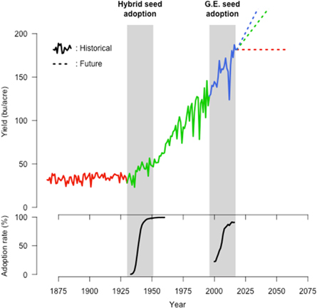
Figure 1. Maize yield trends and technology adoption in the US. The solid line corresponds to historical yields corresponding to three regimes: pre hybrid seed (red), pre-GE seed (green) and post GE seed (blue). The potential future yields under these historical yield regimes are depicted in dashed lines. The periods of hybrid and GE seed adoption are highlighted with the gray band. The adoption 'S'-curves at the bottom correspond to the adoption rate of the corresponding technology (hybrid seed and GE seed). Data sources: USDA/ERS (GE adoption) and USDA/NASS.
Download figure:
Standard image High-resolution imageOur research seeks to inform the technological needs under climate change. More specifically, we aim to distinguish US maize yield trends in the pre- and post-GE era, and contrast these to predicted yield impacts based on climate change models. While the yield differences between these two eras cannot be solely attributed to the adoption of GE seeds, this comparison sheds light generally on the necessary technological advancements required to offset climate change impacts. Here, we provide a novel approach for large-scale estimation of spatially heterogeneous technological effects and climate change impacts simultaneously within a unified econometric model. Importantly, this approach does not require data on actual GE adoption rates, which is typically unavailable or measured at an aggregate level in observational settings, but rather only requires knowledge of when GE varieties became available. Analysis of county-level yields spanning 1981–2015 show that annual yield gains of a similar magnitude as those experienced during the adoption of GE maize are needed to offset climate change impacts under the business-as-usual scenario, and that smaller gains such as those associated with the pre-GE era in the 1980s and early 90s would likely imply yield reductions below current levels. In addition, we show that accurate estimation of historical yield trends requires (i) allowing for a structural break when GE varieties are initially introduced and (ii) controlling for the confounding influence of weather.
The raw data in this study include annual county-level maize yields, monthly precipitation, and daily minimum and maximum temperature observations. We focus on 8 states constituting the US Corn Belt in which GE maize has reached near-complete adoption. The data contain 17 000 observations spanning 500 counties during 1981–2014. As a departure from previous work, we model trends using a piece-wise linear spline with an inflection point in 1996 to allow the trend to vary across the pre-GE (1981–1995) and post-GE (1996–2014) periods. Recent work suggests that yield gains from GE seed adoption have been spatially heterogeneous (Lusk et al 2017), so we rely on hierarchical mixed models with trends varying across agricultural reporting districts within each state. Crop reporting districts are USDA administrative units within each state that contain groupings of counties.
2. Methods
2.1. Data sources
We rely on county-level maize yield data from USDA/NASS (1981–2014). We also rely on average acreage over the sample period as weights for computing aggregate regional impacts. The analysis is based on a balanced panel of 500 counties in eight Midwestern states (Illinois, Indiana, Iowa, Michigan, Minnesota, Missouri, Ohio, and Wisconsin). Maize production in these counties is mostly rain-fed.
For weather data we rely on monthly precipitation and daily maximum, minimum, and average temperature from the PRISM Climate Group (http://www.prism.oregonstate.edu). The PRISM data is a gridded climate dataset with a 4 km spatial resolution that is the official climatological data of the USDA and has been widely used in the climate impacts literature (e.g. Schlenker and Roberts, 2009). The daily PRISM data is available since 1981 and we rely on the 1981–2014 period for our analysis. Daily temperatures are processed into temperature exposure bins of 1 °C each, from −15 °C to 50 °C, which are necessary to estimate nonlinear effects of temperature following Schlenker and Roberts (2009). The temperature exposure data is computed based on a double sine curve passing through the minimum and maximum of each consecutive day at each grid.
Because the analysis is conducted at the county-level, we aggregate the gridded data up to the county level to match the agricultural production data based on the amount of cropland contained in each PRISM grid, which we derive from USDA's 30 m resolution Crop Data Layer.
2.2. Regression models
We specify the statistical model using a linear multilevel model:
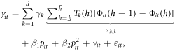
where yit is the natural log of maize yield in county i and year t. The fixed effects portion (in the multilevel model parlance) of the model includes the effects of temperature exposure  and the effects of precipitation
  The random effects captured by vit include random intercepts across counties and random piecewise linear trends across districts:

where t denotes the trend variable with value 16 in the year 1996 and the subscript g denotes ag districts. Parameter estimates are obtained using the lmer function in R and reported in table S1 (available online: stacks.iop.org/ERL/13/124009/mmedia).
All weather variables are aggregated over the April–September growing season following modeling choices in the literature. Our approach is similar to Schlenker and Roberts (2009) in that it allows for nonlinear effects of temperature exposure over the season. More specifically,  is the exposure to temperature bin h over the season, and
  is the element in column k and row h of the basis matrix of a Chebyshev polynomial of degree d defined over temperature bins
  Unless otherwise noted, all models in the study rely on an 8th degree polynomial with
  and
and  so that there is enough exposure at the extreme bins. In a sense, the variable
  is a locally-weighted transformation of temperature bins, which assumes a smooth response to exposure to different temperature levels. We also considered polynomial specifications of various degrees and find the results to be fairly insensitive to the functional form. The effects of precipitation are captured by the inclusion of linear and quadratic terms for seasonal precipitation.
Table S1 shows that the multilevel model produces similar results to the more commonly used panel data 'fixed effects' models used in the literature. The estimated yield-temperature response curve for the multilevel model is similar to those from previous studies (figure S1). We prefer the multilevel model here as it allows for a parsimonious expansion of the trend effects to be heterogeneous across districts, which permits a more localized representation of cross-sectional trend differences compared to previous studies that allow trends to vary at the state-level. This is an important consideration given previous evidence of localized differences in GE adoption effects (Lusk et al 2017).
To represent the variability of estimated effects and projections we rely on a block-bootstrap procedure whereby we estimate the above model 1000 times with data resampled with replacement by year. This follows the bootstrap aggregating or 'bagging' procedure developed commonly used in machine learning (Breiman 1996).
2.3. Climate projections and impacts
The calculation of climate change impacts largely follows the recommendations laid out in Auffhammer et al (2013). Future projections of changes in temperature and precipitation are derived from models archived as part of the Climate Model Intercomparison Project Phase 5 (CMIP5) project, and include the same collection of General Circulation Model (GCM) simulations used for the 5th Intergovernmental Panel on Climate Change (IPCC). Native GCM spatial resolution tends to be between 50–200 km, which is much coarser than required for our estimates of crop yields. The native GCM data is therefore downscaled based on the approach proposed by Mosier et al (2014).
The fine resolution target is the 4 km PRISM grid. The coarse resolution GCM data originate from the IPCC models with surface air temperature (tas), and precipitation (pr) fields available at monthly timescales, and for both historical and climate change scenarios. This list of models is restricted to the following subset of all CMIP5 GCMs: CNRM-CM5, FGOALS-g2, GFDL-CM3, GFDL-ESM2G, GFDL-ESM2M, HadGEM2-CC, HadGEM2-ES, INM-CM4, IPSL-CM5A-LR, IPSL-CM5A-MR, MIROC5, MIROC-ESM-CHEM, MIROC-ESM, MRI-CGCM3, and MRI-ESM1. Several models include multiple ensemble members, and all include simulations of different representative concentration pathways (RCPs). Here, we use the RCP 2.6, 4.5, 6.0 and 8.5 scenarios, which represent total net increase in longwave radiative forcing of 2.6, 4.5, 6.0 and 8.5 W m−2 by the end of the 21st Century, respectively.
Our initial step is to compute historical 'reference' climatologies for each variable at weekly and monthly timescales from each CMIP5 model at its native resolution using the period (of the model) from 1950–2000. Likewise, we compute future climatologies from each GCM for the periods between 2025–2075 and 2050–2100 for each RCP and ensemble. Next, we computed changes in model mean  according to
  for temperature (tas), and
  for precipitation (pr). The changes in temperature are therefore to be regarded as actual differences in the mean and variance of the quantity itself, whereas the changes in precipitation are fractional increases or decreases relative to historical climatology. Changes in mean climatology are computed from each model at each grid point for all ensemble members and scenarios at model resolution prior to interpolation. The final two steps in the downscaling procedure are to (i) interpolate the modified climatologies of the future to the target (4 km) grid, and then (ii) apply those changes to PRISM climatology.
Following the conventional practices in the literature, we calculate county-level climate change impacts on yields in percentage terms as ![$impac{t}_{i}=100(\exp [({{\bf{z}}}_{1{\bf{i}}}\,-\,{{\bf{z}}}_{0{\bf{i}}})\gamma \,+\,({{\bf{p}}}_{1{\bf{i}}}\,-\,{{\bf{p}}}_{0{\bf{i}}})\beta ]\,-\,1)$](https://content.cld.iop.org/journals/1748-9326/13/12/124009/revision2/erlaae9b8ieqn12.gif) where
where  are the baseline temperature and precipitation climate measures and
  are the measures under climate change for each county i. The aggregated impacts for the entire region are the acreage-weighted summation of the county-level impacts.
3. Results
Accounting for weather realizations may be critical for estimating yield trends correctly. Intuitively, a string of peculiar weather realizations could bias the estimation of the trends if such conditions are unaccounted for and materialize disproportionately in either the pre- or the post-GE period. We therefore compare trend estimates using a single linear trend versus a piecewise linear trend with an inflection point at 1996. We also consider random effects for these trends at both the agricultural district and county levels, as well as the inclusion of weather variables as controls. Our preferred model included a piecewise linear trend with random trends at the district level and weather variables included as controls, as it exhibited the lowest AIC (calculated using the approach of Greven and Kneib (2010) for random effects models with the R package 'cAIC4') and similar out-of-sample forecasting accuracy among the alternatives (table S2). We also found that the placement of the knot at 1996 is optimal (figure 2).

Figure 2. Effect of trend inflexion year on model fit. Each bar corresponds to the reduction in Mean Squared Error (MSE) between a model with an inflexion point in the trend, and a model without an inflexion point or weather variables. The year indicates the year of the inflexion of the estimated trend. A higher number indicates a better model fit.
Download figure:
Standard image High-resolution imageWe find maize yield trends increased by almost 70 percent around the period of rapid adoption of GE seeds. We could identify this finding only by accounting for the confounding influence of weather. More precisely, the first two models suggest GE seed adoption did not alter the yield growth trajectory. However, the third model—which predicts yields most accurately—points to large differences in the trend estimates between the pre- and post-GE periods. The trend estimates for the three models are illustrated for the state of Iowa in figure 3 and mirror similar results for other states (figures S2–S8). This finding is consistent with previous work demonstrating the importance of controlling for weather realizations when estimating yield gains from GE adoption (Lusk et al 2017). Since log-yield is the dependent variable in our regression model, the slopes of the piecewise linear trend segments provide an estimate of the annual percentage-change in yields. On average across counties, maize yields grew by 0.94 and 1.59% yr−1 in each of the two periods, indicating GE seed adoption is associated with a net annual yield growth increase of 0.65% points. Given a baseline yield of 120 bushels/acre—approximately the five-year sample-average in these states prior to GE adoption—the compounded gain associated with this technological transition over a 22 year period spanning 1996 to the present is approximately 17.5 bushels per acre. Even though we cannot solely attribute the yield gains to GE seeds alone within our framework, our estimate is strikingly similar in magnitude to estimates based on side-by-side comparisons of GE versus non-GE hybrids in field trials that include cultivar-specific yield observations alongside an extensive set of agronomic and climatic controls (Nolan and Santos, 2012).
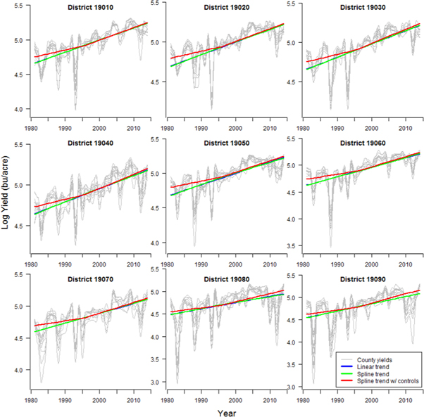
Figure 3. Maize yields and alternative estimated trends by district in Iowa. Each panel portrays yields and estimated yield trends for each agricultural district in the state of Iowa. The gray lines indicate the county-level yields within each district. The blue line represents a linear trend without an inflexion point and without accounting for weather conditions. The green line introduces an inflexion point but does not condition for weather. The red line shows the trend with an inflexion point that accounts for weather conditions. All inflexion points are set at 1996. Results for other states are presented in the appendix.
Download figure:
Standard image High-resolution imageThe trend estimates exhibit extensive cross-sectional heterogeneity. Across counties, the pre-GE trends span 0.64%–1.34% whereas post-GE trends range from 1.07% to 2.15% with pre-post differences ranging between 0.29% and 1.04% points (figures S9–S11). This heterogeneity indicates that technological change has impacted different regions very differently. That is, while new technologies such as GE seeds are widely adopted, benefits can vary substantially across alternative growing conditions associated with local biotic and abiotic factors and interactions thereof.
The effect of climate change on crop yields will severely undercut potential gains from technological progress based on a widely-used GCM. We compare trend estimates with the gross impact of climate change on yields. To ensure comparability we annualize climate change impacts by taking the point-prediction at a given future date divided by the number of years until that date. For example, the total estimated impact is a 77% yield reduction on average across counties for 2050–2100 under the HadGEM2-ES GCM and the business-as-usual RCP 8.5. Annualizing this impact by taking the midpoint of the projection (2075) and benchmarking it to 2010 points to a 1.19% yr−1 reduction.
The combined impact of technological progress and climate change will result in spatially heterogeneous net impacts. Figure 4 illustrates separate county-level annual yield impacts from technology and climate change for the aforementioned climate model and scenario as well as the combined effects. Panels a and b indicate pre- and post-GE trend estimates, whereas panel (c) indicates the gross climate change contribution. Adding the trend estimate to the climate change effect results in the net combined impacts in panels (d) and (e), respectively. The acreage-weighted aggregate trends are 1.02% yr−1 (SE = 0.21) for pre-GE technology; 1.61% yr−1 (SE = 0.22) for post-GE technology; and −1.14% yr−1 (SE = 0.10) for climate change. The aggregate combination of the trend plus climate change impacts are −0.12 (SE = 0.24) and 0.47% yr−1 (SE = 0.25) for pre- and post-GE, respectively. These results are naturally sensitive to the GCM and the RCP scenario. For example, under the CNRM-CM5 climate model and RCP 8.5 scenario, the combined impacts are 0.25 and 0.90% yr−1 for the pre- and post-GE technologies (figure S12). If instead, we hold the GCM fixed and consider the lowest emissions trajectory (i.e. HadGEM2-ES, RCP 2.6), the combined impacts are 0.58 and 1.2% yr−1, respectively (figure S13).
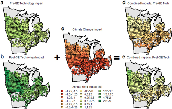
Figure 4. Decomposition of annualized projected yield effects for the Midwest. Each panel corresponds to an annualized percentage yield impact for each county of (a) technological progress based on the pre-GE trend (1981–1995), (b) technological progress based on post-GE trend (1996–2014), (c) the impact of climate change (HadGEM2-ES, RCP 8.5, 2050–2100), (d) the combined impacts of pre-GE trend and climate change and (e) the combined effect of post-GE trend and climate change.
Download figure:
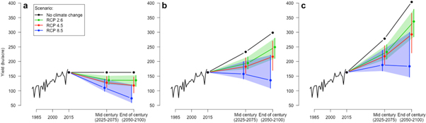
Standard image High-resolution imageClimate change will severely curtail potential crop yield gains from technological progress in the coming decades based on a wide range of GCMs. Yield projections under all of the GCMs in CMIP5 and RCPs are provided in figure 5 for three different regimes: no yield growth (panel (a)), yield growth comparable to pre-GE era (panel (b)), and yield growth comparable to post-GE era (panel (c)). Under the RCP 8.5 scenario, it will take innovations on the order of the post-GE era to offset climate change impacts. Yield gains less than that, such as those exhibited prior to GE adoption, would lead to reductions in yield levels by the end of the century. Mitigation of CO2 emissions under the 2.6 and 4.5 RCPs point to a much more optimistic outlook as projected yields would continue to rise through the end of the century under both the pre- and post-GE technological regimes.
Figure 5. Historical and projected maize yields under alternative growth regimes and climate scenarios. (a) No growth in yields, (b) continued pre-GE growth in yields, and (c) post GE growth in yields. The black line prior to 2015 corresponds to the historical yield trend. The black line beyond 2015 corresponds to the projected yield level without climate change under a given yield growth regime. The colored dots and bars represent the CMIP5 ensemble mean and extrema for the middle and end of the century for 3 different climate scenarios. The colored band are added to improve readability.
Download figure:
Standard image High-resolution image
4. Discussion and conclusion
US Maize yields exhibit sustained growth since the adoption of hybrid seeds in the 1930s. We find that this growth has accelerated with the adoption of GE seeds, and that this acceleration can only be fully appreciated when accounting for weather patterns which can be confounded with secular technological trends. We cannot identify the biophysical source of this acceleration, but our findings are consistent with yield gains attributed to GE maize adoption in analyses based on both experimental field-trial and actual on-farm yields (Lusk et al 2017). While GE traits do not necessarily increase the maximum possible yields (i.e. yield potential), they have been associated with narrowing yield gaps through improved weed control, insect resistance, and more timely planting (Fisher and Edmeades 2010).
Our results suggest that the relative increase in maize yields has been nonlinear since 1980, with a clear structural change in the growth rate occurring in 1996. Although much recent literature suggests a linear growth trend over many decades for US maize yields (Cassman et al 2011, Grassini et al 2013), our findings are more in line with studies having identified a nonlinear change in yield trends attributed to GE adoption (Fischer and Edmeades 2010, Xu et al 2013, Lusk et al 2017). Our analysis suggests that controlling for weather outcomes when estimating yield trends is crucial, and would likely resolve existing debate regarding the appropriateness of linear trend assumptions.
The growth rate of crop yields in the coming decades will have serious implications for the global food supply under climate change. Our results suggest that US maize yields could stagnate under a business-as-usual scenario even with bold assumptions about the sustained growth in crop yields. This has serious implications for other crops and countries as well, as there are many large, economically relevant regions in the world where technology adoption lags and the use of GE crops are prohibited (Barrows et al 2014). In addition, GE varieties of rice and wheat are not commercially available. If the relative yield gains estimated here are any indication of the potential for other crops and/or regions, then the adoption of new technologies such as GE varieties may constitute a potentially fruitful adaptation strategy for counterbalancing the effects of climate change. Consumer preferences for (or against) will continue to play a critical role in the global pattern of land-use for production of GE crops and have the potential to alter trade patterns among countries (Garrett et al 2013, VanWey and Richards 2014).
Our findings also provide key implications for research and development. Emerging technologies in genome editing as well as an increased emphasis on abiotic stress tolerance (e.g. drought tolerance) could help maintain or even accelerate recent yield growth trends (Parisi et al 2016, Svitashev et al 2016). In addition, the rise in computing power and fine-scale data collection and analysis may pave the way for a digital revolution that may also contribute to such trends through enhanced precision agriculture. It remains to be seen whether these technological revolutions and the legal framework to reward such innovations and protect intellectual property rights will unfold rapidly enough to counterbalance the projected effects of a changing climate.
Finally, our study has some caveats that bear mentioning. First, while our trend analysis identifies a yield trend increase around the time of rapid adoption of GE seeds, our study is unable to identify the biophysical source of this change. There could be other confounding factors that generated yield gains parallel to the introduction of GE maize in the US such as the adoption of precision agricultural tools such as high-speed precision planters and auto-steer tractors. We consider the possibility of an increase in solar radiation and find that our results are robust to controlling for increased levels of solar brightening (Tollenaar et al 2017) that occurred over the sample period (figures S14–S16). Second, our climate change projections do not factor in fertilization effects of increased atmospheric CO2 levels (Urban et al 2015), nor behavioral adaptation to climate change (Butler and Huybers 2013, Burke and Emerick 2016). These additional factors could result in potentially more optimistic impacts.
Author contributions
AOB collected the data and processed the weather variables and climate predictions. JT and AOB contributed equally to all other aspects of the research. Senior authorship is shared equally.
Acknowledgments
AOB was supported by NSF grant 1360424. We thank Carlos M Carrillo for providing the downscaled climate projections.