


Abstract
Aboveground biomass (AGB) estimates for regional-scale forest planning have become cost-effective with the free access to satellite data from sensors such as Landsat and MODIS. However, the accuracy of AGB predictions based on passive optical data depends on spatial resolution and spatial extent of target area as fine resolution (small pixels) data are associated with smaller coverage and longer repeat cycles compared to coarse resolution data. This study evaluated various spatial resolutions of Landsat-derived predictors on the accuracy of regional AGB models at three different sites in the eastern USA: Maine, Pennsylvania-New Jersey, and South Carolina. We combined national forest inventory data with Landsat-derived predictors at spatial resolutions ranging from 30–1000 m to understand the optimal spatial resolution of optical data for large-area (regional) AGB estimation. Ten generic models were developed using the data collected in 2014, 2015 and 2016, and the predictions were evaluated (i) at the county-level against the estimates of the USFS Forest Inventory and Analysis Program which relied on EVALIDator tool and national forest inventory data from the 2009–2013 cycle and (ii) within a large number of strips (~1 km wide) predicted via LiDAR metrics at 30 m spatial resolution. The county-level estimates by the EVALIDator and Landsat models were highly related (R2 > 0.66), although the R2 varied significantly across sites and resolution of predictors. The mean and standard deviation of county-level estimates followed increasing and decreasing trends, respectively, with models of coarser resolution. The Landsat-based total AGB estimates were larger than the LiDAR-based total estimates within the strips, however the mean of AGB predictions by LiDAR were mostly within one-standard deviations of the mean predictions obtained from the Landsat-based model at any of the resolutions. We conclude that satellite data at resolutions up to 1000 m provide acceptable accuracy for continental scale analysis of AGB.
Export citation and abstract BibTeX RIS

Original content from this work may be used under the terms of the Creative Commons Attribution 3.0 licence.
Any further distribution of this work must maintain attribution to the author(s) and the title of the work, journal citation and DOI.
Introduction
Large scale estimates of aboveground biomass (AGB) in a periodic and consistent fashion is critical for understanding forest structure and productivity and implementing strategic policies such as carbon emission mitigation under the United Nations Framework Convention on Climate Change (UNFCCC). The US Department of Agriculture Forest Service (USFS) conducts annual forest inventories and produces statewide and national estimates of carbon stocks and stock changes following a consistent sampling design and protocols established under the national Forest Inventory and Analysis (FIA) program (Heath et al 2011). The FIA program provides strategic-level data from permanent sample plots distributed over all land cover types and ownerships. However, the FIA design-based estimates from the strategic scale of inventory are reliable only to larger spatial scales such as county-level (McRoberts 2008) because the distribution of field plots is relatively sparse and inadequate for small-area (e.g. forest stands) estimation. Further, studies based on FIA data across large domains of space and time often encounter constraints because of inconsistent sampling methods (e.g. intensity) and insufficient or no field data (e.g. interior Alaska). A sufficient number of representative sample plots can provide reliable estimates of AGB, relying on extant allometric models and expansion factors for the sampling measurements. The FIA program has established at least one plot per 2400 ha of land, and sufficient number of plots for large-area estimates are determined based on sampling error standards as defined in the database description and user guide (Burrill et al 2017, McRoberts 2008).
Satellite imagery integrated with the annual national forest inventory data have the potential to extend the sample plot attributes over large spatial (wall-to-wall) and temporal scales. The systematic, synoptic, and spatially complete characteristics of satellite sensors along with free and open access to data sources and processing/analysis opportunities have enabled a reliable and cost-effective estimation of AGB and carbon over large-areas in contrast to those solely based on field data. In addition, availability of free Landsat imagery in analysis-ready formats facilitates large area forest dynamics analyses at spatial resolutions consistent with operational requirements for resource managers. Landsat imagery is globally captured at 30 m spatial and ~16 day temporal resolutions via consistent bandwidths of multiple sensors since 1984, and systematically rectified data are publicly available from the archive of US Geological Survey (Banskota et al 2014). This characteristic of Landsat data enables national scale ecosystem monitoring and study of biomass dynamics in a systematic and repeatable fashion (Wulder et al 2012). The fine spatial resolution of Landsat data is more likely to reduce uncertainty in AGB estimates because structural and compositional variability over a landscape are better represented in 30 m pixels (Brosofske et al 2014, White et al 2016) than in coarse resolution data such as MODIS imagery at 250–1000 m resolutions (https://modis.gsfc.nasa.gov/). Another reason for less uncertainty with Landsat data is the compatible sizes of image pixels and ground sample plots in most national forest inventories, in contrast to coarse resolution data that record mixed spectral signatures within a pixel. Satellite data with wider spatial coverage and higher temporal resolutions (e.g. 2330 km swath width and 1–2 days temporal frequency of MODIS imagery) are further enriching the domain of spatial predictors for regional scale estimation of AGB; however, their coarse resolutions impair the sensitivity of predictors for AGB. The time-series data of multiple sensors can also help reduce the impact of clouds and aerosol contamination since the best available pixel can be selected as the predictor variable (White et al 2014). Nonetheless, there are tradeoffs in the prediction accuracy versus operational efficiency of optical data as high spatial resolutions have to compromise with low temporal resolutions of sensors.
Periodic mapping of AGB at a shorter time steps (e.g. annual) over larger areas (e.g. statewide) using Landsat-derived predictors can be unrealistic because of the longer repeat cycle (~16 day) and prevalence of extensive atmospheric noise in the spectral signals. In addition, the need for leaf-on or growing-season imagery to capture the spectral response of broadleaves reduces the list of suitable Landsat imagery for a season in a year. However, such a problem can be solved with MODIS data because of high imaging frequency (i.e. every other day) and similar or better radiometric resolutions compared to Landsat. The larger pixels of MODIS data do not necessarily mean that pixel-level AGB prediction is invalid. For example, Chen et al (2016) reported that when LiDAR-derived grid metrics were aggregated to coarser resolutions (from 13 m up to 390 m), pixel-level relative AGB prediction error decreased initially and then flattened, and model predictors made a small contribution to the total error in the predictions across different cell sizes. A noted drawback of passive optical sensors is the issue of signal saturation in high biomass areas with stocks above 300 Mg ha−1 (Zhang et al 2014). LiDAR technology has evolved in the past three decades because this active remote sensing system provides an accurate three-dimensional profile of forest structure and the metrics have been found to be highly related with AGB and other structural attributes (Deo et al 2016). While multispectral data provide two-dimensional information on canopy coverage, integration of height information from active sensors such as LiDAR has the potential to improve AGB prediction accuracy. However, LiDAR data cannot replace (but augment) ground observations and need representative sample plots to develop AGB prediction models (Nelson et al 2017).
The effects of predictors' grid size and field plot configuration on the uncertainties of LiDAR-based models have been reported in several studies (Hayashi et al 2016, Tomppo et al 2016). However, optical satellite data that provide wide and synoptic coverage have not been evaluated in any of the past studies for the impact of pixel size on the AGB prediction estimates. Unlike in small-scale operational planning, regional- or national-scale forest carbon estimation may not necessarily require a high resolution AGB map (Blackard et al 2008, Chen et al 2016). A regional or national scale spatial inventory of AGB can be made via a generic model selected for a diverse range of forests (Deo et al 2017) and coarse resolution spatial predictors can satisfy the accuracy standards for national reporting and related strategic planning. For example, if MODIS data at 250 m spatial resolution and near daily repeat cycles produce accuracies similar to Landsat data at 30 m resolution, then the issue of data gap can be avoided. Additionally, intensive processing and modeling time/efforts required with 30 m resolutions of Landsat data can be minimized with aggregated pixels at a coarser resolution.

Figure 1. Location of the study sites in Maine (ME), Pennsylvania-New Jersey (PANJ) and South Carolina (SC) across the eastern USA. The vertical and horizontal bands are LiDAR strips acquired under a carbon monitoring system (CMS) program that also conducted independent field plot measurements in 2014 within the strips.
Download figure:
Standard image High-resolution imageThe objective of this study was to evaluate the accuracy of AGB models for large-area estimation based on a range of spatial resolutions of Landsat-derived predictors. To optimize the spatial resolution of predictors for large area AGB estimation, we further evaluated how well county-level estimates provided by models at various spatial resolutions compared with the design-based estimates of FIA field inventories. Since LiDAR based models are known to produce high accuracy in AGB estimation, we also compared the predictions for wide strips (~1 km) where extant AGB estimates are available (Deo et al 2017).
Methods
Study area
The study area is comprised of three sites represented by Landsat scene WRS-2 path/rows of 14/32, 12/28 and 16/37 over Maine (ME), Pennsylvania- New Jersey (PANJ), and South Carolina (SC), respectively, across the eastern USA (figure 1). The sites differ considerably in forest structure and composition due to substantial differences in geoclimatic characteristics and variations in forest management practices. Average annual temperatures are 5.2, 10.6 and 18.2 °C and average annual precipitations are 117, 123, and 120 cm for ME, PANJ and SC, respectively. The terrain elevations range from 98–1138, 0–674, and 0–114 m above sea level in ME, PANJ, and SC, respectively. The sites differ in species composition that characterize boreal and eastern deciduous forests in ME (McCaskill et al 2011) and loblolly-shortleaf pine, oak-hickory and oak-gum-cypress forest-type groups in SC (Rose 2016). Mixed-oak, northern hardwoods and loblolly/ shortleaf pine are the dominant forest-type groups in the PANJ site (Crocker 2014, McCaskill et al 2013).
Remotely sensed data
Landsat-8 surface reflectance images captured by Operational Land Imager (OLI) sensor during the peak growing seasons (July and August) of 2014, 2015 and 2016 that contained less than 5% cloud cover per scene were acquired from the USGS Climate Data Records (CDR 2017) via the ESPA on demand interface (https://espa.cr.usgs.gov). The sites required 9, 7 and 8 scenes in ME, PANJ and SC, respectively to cover the entire study area (supplementary table 1 available at stacks.iop.org/ERL/13/055004/mmedia). The high-level image products from the CDR included blue, green, red, near infrared and shortwave infrared surface reflectance bands in addition to other derived metrics and vegetation indices as described in Deo et al (2017). Any cloud- and shadow-affected areas of the raster layers were masked out before using them as predictors in AGB estimation. There were altogether 19 spatial predictors at the original spatial resolution of 30 m that were subsequently resampled to 60, 90, 120, 150, 250, 300, 500, 750 and 1000 m spatial resolutions (accordingly matching ~2 × 2, 3 × 3, 4 × 4, 5 × 5, 8 × 8, 10 × 10, 17 × 17, 25 × 25 and 33 × 33 windows of 30 m pixels) via the aggregate function in ArcGIS that yielded mean input values to the output pixel.
Field data for model training
The field data for model training were based on the FIA plots measured in 2014, 2015, and 2016 within each of the study sites. The plots were selected so that the year of plot measurements and Landsat observations matched. There were 3849 plots of which 1766 were in ME, 675 in PANJ, and 1408 in SC. The FIA plot data for each site were attached to the co-located 19 predictors at each of the 10 spatial resolutions, and 10 generic reference (training) data frames (corresponding to each of the resolutions) were created by pooling over all plots at the three sites. In the spatial joining of plot data with the fine resolution predictors at 30 m grid (pixel), mean spectral values of predictors from the 3 × 3 pixel-window around the central subplot was used because the FIA plot configuration consisting of four subplots spread over a square block of nine 30 m pixels. The plot AGB was calculated following the methods in Jenkins et al (2003) which first employed allometric models to determine individual tree biomass. The mean AGB values for the plot observations were 78.04, 136.57 and 97.36 Mg ha−1 and standard deviations were 43.99, 102.43 and 52.56 Mg ha−1 in ME, PANJ and SC, respectively.
Modeling and validation
Deo et al (2017) demonstrated that a generic model combining data from multiple sites produces comparable or even better accuracy than site-specific models developed from local data only. So, a generic model for each of the 10 resolutions was developed after removing collinear and insignificant predictors (Deo et al 2017). A multivariate variable screening based on QR-decomposition, random forest based model selection, and forward-backward stepwise regression methods were followed to obtain a parsimonious set of significant predictors for each training data frame. The optimal sets of predictors selected were used in ordinary least squares multiple linear regressions (MLR) to construct AGB models for each of the resolutions. The model accuracies were noted in terms of coefficient of determination (R2) and root mean square error (RMSE).
The 10 AGB models were applied to each of the sites to obtain estimates at different resolutions (raster outputs). The prediction estimates were evaluated at the county-level against the design-based estimates by the USFS EVALIDator tool (Forest Service 2015) using the FIA plots measured during the 2009–2013 cycle, prior to the measurements of training plots in 2014, 2015 and 2016. Additionally, large-area prediction estimates were compared with existing AGB estimates based on LiDAR metrics at 30 m spatial resolution for linear strips of about 1 km width for the same sites (Deo et al 2017). The accuracies of predictions by each of the models for the county scale and within the widths of LiDAR strips were calculated in terms of mean deviation (i.e. bias), RMSE and Pearson's correlation (r) amongst the predictions and the references (i.e. EVALIDator and LiDAR strip estimates). The bias, RMSE, standard error (SE) and correlation of predictions and observations at pixel/plot-level were also calculated using an independent set of plot data (see, Deo et al 2017). The independent set of plots was located only within the LiDAR strips (figure 1).
Table 1. Fit statistics of the aboveground biomass (AGB) models at various spatial resolutions of Landsat predictors, and validation statistics based on the comparison of observed and predicted AGB at the independent plot locations.
| Grid size (m) of model predictors | Model RMSE (Mg ha−1) | Model Adj. R2 | Significant variables in the model selectiona | Validation statistics based on the model predictions and observations (Mg ha−1) at independent plots for all three sites combined | |||
|---|---|---|---|---|---|---|---|
| RMSE | SE | bias | r | ||||
| 30 | 64.38 | 0.229 | B3, B6, EVI, MSAVI, NDVI, SAVI, TCG, TCW | 69.34 | 5.39 | 24.83 | 0.58 |
| 60 | 65.27 | 0.207 | B2, B3, B7, EVI, MSAVI, NBR, NBR2, NDVI, SAVI, TCG, IFZ | 71.40 | 5.55 | 27.20 | 0.59 |
| 90 | 65.58 | 0.199 | B2, B3, B7, EVI, MSAVI, NDMI, NDVI, SAVI, TCG, IFZ | 72.73 | 5.59 | 28.50 | 0.56 |
| 120 | 66.45 | 0.178 | B3, B5, EVI, MSAVI, NBR, NBR2, NDVI, SAVI, TCB, TCW, IFZ | 74.32 | 5.64 | 29.95 | 0.53 |
| 150 | 66.66 | 0.173 | B3, B6, EVI, MSAVI, NBR, NDVI, SAVI, TCG, TCW, IFZ | 74.67 | 5.74 | 31.03 | 0.55 |
| 250 | 67.93 | 0.141 | B3, B5, EVI, MSAVI, NDMI, NDVI, SAVI, TCB, TCW | 75.89 | 5.75 | 33.10 | 0.54 |
| 300 | 68.26 | 0.133 | B3, B5, EVI, MSAVI, NDMI, NDVI, SAVI, TCB, TCW, IFZ | 76.55 | 5.78 | 33.29 | 0.54 |
| 500 | 68.78 | 0.119 | B3, B5, EVI, MSAVI, NDMI, NDVI, SAVI, TCA, TCB, TCW, IFZ | 79.50 | 5.92 | 37.11 | 0.51 |
| 750 | 69.60 | 0.098 | B3, B5, EVI, MSAVI, NDMI, NDVI, SAVI, TCB, TCW, IFZ | 83.29 | 6.32 | 35.42 | 0.34 |
| 1000 | 69.89 | 0.091 | B2, B3, B5, B7, MSAVI, NBR2, NDVI, SAVI, TCB, DI, IFZ | 80.78 | 6.02 | 36.91 | 0.48 |
aThe individual predictors are as follows: B2- band2 or blue band, B3- band3 or green band, B5- band5 or near infrared band, B6- band6 or shortwave infrared 1 band, B7- band7 or shortwave infrared 2 band, NDVI- normalized difference vegetation index, NDMI- normalized difference moisture index, EVI- enhanced vegetation index, SAVI- soil adjusted vegetation index, MSAVI- modified soil adjusted vegetation index, IFZ- integrated forest z-score, TCB- tasseled cap brightness, TCG-tasseled cap greenness, TCW-tasseled cap wetness, and TCA- tasseled cap angle (see, Deo et al 2017).
Results
The accuracy of models decreased with increasing pixel size of the predictors (table 1). The coefficient of determination (adj. R2) and RMSE of the model fits, in addition to the validation statistics based on the comparison of plot-level predictions against independent observations at the independent plot locations revealed reduced accuracy with increasing pixel size. Although the fit and validation statistics reveal that the fine resolution predictors (e.g. those <90 m) produce more accurate models, statistics such as correlation and SE from the plot-level observations and predictions at the sites were similar across all models (table 1). The final (optimal) set of spatial predictors found in the model selection process were not consistent across the spatial resolutions, however, the green band and normalized difference vegetation index were in general the best predictors (table 1; supplementary figure A).
The comparisons of average AGB estimates in the strips of LiDAR coverage indicated that the Landsat model based on covariates at 30 m pixels provided estimates closest to that based on LiDAR models (also via 30 m grid metrics) from Deo et al (2017) (figure 2, supplementary table 2). The mean of AGB predictions by LiDAR metrics in the strips are mostly within one-standard deviations of the mean predictions obtained from the Landsat-based model at any of the resolutions. The standard deviation of the Landsat based models decreased with increasing grid size of the predictors (figure 2). The Landsat based average estimates were larger than the LiDAR based average estimates in the strips and the difference ranged from 2–34 Mg ha−1.
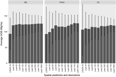
Figure 2. Average AGB estimates (Mg ha−1) in the strips of LiDAR coverage by LiDAR metrics at 30 m resolution (obtained from Deo et al 2017) and the Landsat based models of various resolutions. The error bars represent one standard deviation above and below the mean of predictions. Lsat is short form for Landsat.
Download figure:
Standard image High-resolution imageThe relationships between county-level total AGB estimates by the EVALIDator and the Landsat models were strong (R2> 0.66) at all of the resolutions. However, the strengths of these relationships varied with sites as revealed by the R2, RMSE and slope of the linear fit between the two sets of predictions (i.e. by the EVALIDator and Landsat models; supplementary table 3). The total AGB estimates from the Landsat-based models were higher than the EVALIDator-based estimates as revealed by all slopes <1 in the regression between EVALIDator and Landsat AGB estimates (supplementary table 3). The RMSEs obtained from the two sets of county-level total predictions were also found to be stable across the model resolutions.

Figure 3. Scatter plot of independent plot-level observed versus predicted AGB values (Mg ha−1) using 30 m, 250 m and 500 m resolutions of Landsat predictors. The solid inclined line represents 1:1 line.
Download figure:
Standard image High-resolution image
Discussion
The combined strength of optical remote sensing and field sample data has been demonstrated in many published studies on AGB estimation (Deo 2014). Fine resolution spatially explicit (wall-to-wall) inventories based on Landsat data combined with field plot measurements have operational advantage compared to the traditional inventories employing field data alone. However, the accuracy of Landsat-based approaches to inventory modeling depends on several factors such as sensitivity of image bands to the variation in forest structure and characteristics of the field sample data. As satellite data of coarser resolutions are associated with higher temporal resolutions, periodic mapping of AGB over regional or continental scales is realistic since most data are available in analysis-ready format or less processing efforts are involved. Considering the research need, this study evaluated the impact of spatial resolution of Landsat derived predictors on large-area AGB estimation to support national strategic plans.
The large-area estimates (e.g. county-level) using predictors at 30–1000 m spatial resolutions produced high correction with EVALIDator-based inventory estimates. An inference from this observation is that strategic plans requiring regional- or continental-scale estimates of AGB can rely on moderate to coarse resolution satellite products (e.g. MODIS derived indices and composites). Since finer resolution data such as from Landsat and Sentinel-2 require extra processing efforts and cloud-free data may be unavailable at a given time for an area of interest, coarse resolution predictors are essential to conduct regular assessments such as at annual time steps. However, small-area (e.g. stand-level) assessments based on coarse resolution data may not serve the operational management goals as the sensors are inefficient to capture the spatial variability of forest structure, render mixed pixel effects, and possess limited power for discriminating species and cover types. The operational inventory systems may require methods of local relevance with qualities of cost-efficiency and reliability (White et al 2016). Hence active sensors such as LiDAR and photogrammetric methods based on high resolution passive optical imagery are getting wider attention in the remote sensing community and forest managers for operational applications. Since several public and private agencies are involved in acquiring large area LiDAR datasets, and metrics are even in the public domain, highly accurate small-scale assessments are possible with such data.
The coefficients of determination of the fitted models were comparatively low (R2 < 0.23) and that can be associated to factors such as spatial mismatch of FIA plots and corresponding pixels in the predictors, incompatible size of the plots and pixels, radiometric variations within and among adjacent scenes, and mixed pixel effects in coarse resolution predictors (Pond et al 2014, Tomppo et al 2008). The large structural and compositional diversity of forests within and across the sites combined with the effect of Landsat signal saturation in high biomass areas can be associated with the low prediction accuracies of models at plot-level. The 95th percentiles of the observed AGBs in the FIA plots were 331.3, 388.6, and 406.1 Mg ha−1 while Landsat signals generally saturated near 200 Mg ha−1 (figure 3). The FIA plot design also caused inconsistency for the fine (e.g. 30 m) and coarse (>120 m) pixel sizes because the four subplots (7.3 m radius) in an FIA plot are very small, and spread over about an area of about one acre. The individual subplots in an FIA plots may be differently stocked while Landsat predictors provide a single spectral signature for a plot. When the pixels are aggregated to coarser sizes, diverse spectral signatures of neighboring pixels are subject to spectral smoothing. As expected the standard deviation of the Landsat based predictions decreased with increasing grid size of the predictors (figure 2) because of the smoothing effect of spectral signatures with pixel aggregations. Further, the standard error of Landsat estimates were less than the LiDAR estimates and the error decreased with increasing grid size given the large number of cells in high resolution maps. Chen et al (2016) also observed that the prediction error decreased with increasing grid size of predictors.
The increasing grid size of Landsat metrics resulted in slightly increasing estimates of AGB density (figure 2) which can be related to the effects of regression towards the mean and reduced values of R2 with the increasing grid sizes for model fittings. For example, when the models were applied to obtain predictions at the independent plot locations to compare with corresponding field observations, over-estimation was noticed in plots with low biomass areas and under-estimation in high biomass areas (figure 3). Since low biomass areas dominate over the landscape compared to high biomass areas, over-estimation in the study can be related to the effects of regression towards the mean. Hayashi et al (2016) also observed increasing trend of stand-level estimates with a larger grid size of predictors. The saturation of canopy-reflectance and biomass relationship above a certain threshold in high biomass areas leads to spatial models that generate estimates closer to the mean at every pixel (i.e. over-prediction in areas of low biomass and vice-versa). A regression towards the mean effect was obvious as prediction for plots with high observed AGB density saturated above 200 Mg ha−1, while low density plots were over-predicted (figure 3). The root mean square errors of plot-level predictions are consistent with other studies as reported in Deo et al (2016).
The EVALIDator-based county-level total estimates of AGB were found to be consistently lower than the Landsat based predictions (supplementary table 3) because EVALIDator generates estimates only for the forested areas defined as areas with more than 10 percent crown cover, at least one acre in size and 120 feet wide; while Landsat model gave predictions without any restriction to this definition of forest.
Conclusions
Landsat-based spatial AGB models at resolutions ranging from 30–1000 m were developed using FIA data and the prediction estimates were compared with existing large-area reference estimates (i.e. forest inventories) and an extant AGB map based on LiDAR metrics. All the AGB estimates produced at the various resolutions were highly correlated with the forest inventory estimates and LiDAR-based models. The RMSE and bias from the difference of the county-level estimates by the forest inventory and Landsat models were stable across all the spatial resolutions. The Landsat-based average estimates in the strips of LiDAR coverage were very close to the average obtained based on LiDAR metrics, i.e. one standard deviation above and below the average estimate produced by the LiDAR metrics included the averages obtained from the Landsat models. We conclude that the AGB models based on the native (30 m) and coarser resolutions of Landsat-derived predictors provide similar estimates for continental scale analyses.
Acknowledgments
This work was supported by the US Department of Agriculture Forest Service Information Resources Direction Board through the Landscape Change Monitoring System and the NASA Carbon Monitoring System (NASA reference number: NNH13AW62I), in addition to the US Forest Service—Northern Research Station (#14-JV-11242305-012), and the Minnesota Agricultural Experiment Station (project MIN-42-063). We thank three external reviewers for their comments that improved this manuscript.