

Abstract
This study examines underlying reasons for differences among land-based greenhouse gas flux estimates in Indonesia, where six national inventories reported average emissions of between 0.4 and 1.1 Gt CO2e yr−1 over the 2000–2012 period. The large range among estimates is only somewhat smaller than Indonesia's GHG mitigation commitment. To determine the reasons for these differences, we compared input data and estimation methods, including the definitions and assumptions used for setting accounting boundaries, including emitting activities, incorporating fluxes from various carbon pools, and handling legacy fluxes. We also tested the sensitivity of methodological differences by generating our own reference emissions estimate and iteratively modifying individual components of the inventory. We found that the largest changes stem from the inclusion of legacy GHG emissions due to peat drainage (which increased emissions by at least +94% compared to the reference), methane emissions due to peat fires (+35%), and GHG emissions from belowground biomass and necromass carbon pools (+61%), modifications to assumptions of the mass of fuel burnt in peat fire events (+88%), and accounting for regrowth following a deforestation event (−31%). These differences cumulatively explain more than half of the observed difference among inventory estimates. Understanding the various approaches to emissions estimation, and how these influence the magnitude of component GHG fluxes, is an important first step towards reconciling GHG inventories. The Indonesian government's success in achieving its mitigation goal will depend on its ability to measure progress and evaluate the effectiveness of abatement actions, for which reliable harmonized greenhouse gas inventories are an essential foundation.
Export citation and abstract BibTeX RIS
1. Introduction
At the Paris Conference of Parties to the United Nations Framework Convention on Climate Change (UNFCCC) in 2015, 195 countries committed to reduce anthropogenic greenhouse gas (GHG) emissions (UNFCCC 2016). Land use, land use change, and forestry (LULUCF) features prominently in the Paris Agreement, with 83% of countries including mitigation actions in this sector in their Nationally Determined Contributions (NDCs) (FAO 2016). Collectively, these activities are expected to contribute up to one-quarter of all pledged emissions reductions (Forsell et al 2016, Grassi et al 2017). Despite their importance, LULUCF emissions and removals remain the most uncertain component of the carbon budget (Houghton et al 2012). The range of published estimates of global LULUCF fluxes differ by up to a factor of two (Pongratz et al 2014), and these discrepancies can be even larger at the scale of individual countries (Roman-Cuesta et al 2016).
Underpinning the success of mitigation actions such as those outlined in the NDCs are reliable national GHG inventories. The Intergovernmental Panel on Climate Change (IPCC) provides guidance for producing unbiased GHG inventories that are reported in a transparent way, and are complete, comparable, consistent over time, and accurate (collectively, these are referred to as the TCCCA principles) (IPCC 2003, 2006a, 2013). There has been growing focus on improving the accuracy of LULUCF GHG inventories by investing in data collection, including mapping land cover and land conversion, and measuring corresponding GHG fluxes (Baker et al 2010, GOFC-GOLD 2016). However, the underlying reasons for differences among GHG flux estimates go beyond documented challenges with respect to input data measurement and accuracy (Pongratz et al 2014). In calculating LULUCF GHG fluxes, there are many acceptable methodological alternatives which may be motivated by various policy questions, and which produce different results. Recent studies suggest that the magnitude of disagreement in inventory GHG flux estimates introduced by these alternative assumptions, definitions, and degrees of inventory completeness, rivals the scale of uncertainty associated with input data (Federici et al 2017, Houghton et al 2012, Milne and Grubnic 2011, Pelletier et al 2013).
For example, Pongratz et al reported that the two-fold difference in published estimates of global LULUCF fluxes is largely the result of variable treatment of land use feedbacks, carbon sinks, and legacy carbon fluxes (Pongratz et al 2014). Another study determined that the discrepancy between Harris et al's estimate of 3.0 Gt CO2e yr−1 due to pan-tropical deforestation (Harris et al 2012b), and Baccini et al's estimate of 8.1 Gt CO2e yr−1 (Baccini et al 2012), is due to differences in the scope of activities and carbon pools included, the spatial scale of analysis, and whether emissions were modeled over time or assumed to occur instantaneously (Harris et al 2012a). Similarly, Calle et al found that the differences between published estimates of GHG flux across Asia, which range from a net sink of −0.6 Gt CO2e yr−1 to net source of 1.5 Gt CO2e yr−1 for the 2000s, can be attributed to different decisions about if and how to incorporate various flux components (Calle et al 2016).
Despite the impact of alternative methods, assumptions, and definitions on the wide range in reported global and regional GHG fluxes, there have been few studies of their impacts on national GHG inventory estimates. The present study examines the underlying reasons for differences among LULUCF GHG inventories, using Indonesia as a case study. Indonesia ranks among the top ten GHG emitters in the world (CAIT 2014), and at least 40% of national emissions derive from LULUCF activities (Republic of Indonesia 2016a). However, there are six recent government-led GHG inventories that have reported average annual emissions from LULUCF of between 0.4–1.1 Gt CO2e yr−1 over the 2000–2012 period (figure 1). The discrepancy between the lowest and highest reported estimate is 0.7 Gt CO2e, a difference only somewhat less than the country's NDC commitment to unconditionally reduce GHG emissions by 29%, or 0.8 Gt CO2e, below a projected baseline by 2030 (Republic of Indonesia 2016a).

Figure 1. Reported estimates of land-based GHG fluxes in Indonesia from six national inventories.
Download figure:
Standard image High-resolution imageTable 1. List of inventories included in this assessment, and their purpose and funding source. We include a simplified inventory name used to refer to each inventory in this paper.
| Inventory name | Purpose | Funding source | Reference |
|---|---|---|---|
| FREL 2014 | Establishment of a national forest reference emissions level (FREL), per Minister of Forestry Decree 633/2014. | NORAD | Sugardiman et al (2014) Setting forest reference emissions level for Indonesia. Directorate General of Forestry Planning, Ministry of Forestry and the Center for International Forestry Research, Bogor, Indonesia. |
| BP REDD+ 2015 | Development of national forest reference emission level (FREL) for deforestation and forest degradation in the context of results-based payments for REDD+, according to UNFCCC decision 12/CP.17. | Norwegian Government funding through the UNDP | BP REDD+ (2015) National Forest Reference Emission Level for Deforestation and Forest Degradation in the Context of the Activities Referred to in Decision 1/CP.16 para 70 under the UNFCCC. BP REDD+, Jakarta, Indonesia. |
| INCAS 2015 | Development of national platform for greenhouse gas accounting to meet measurement, reporting and verification (MRV) requirements in the land based sectors. | Australian Government | Krisnawati et al (2015) National Inventory of Greenhouse Gas Emissions and Removals on Indonesia's Forests and Peatlands. Research, Development and Innovation Agency of the Ministry of Environment and Forestry, Bogor, Indonesia. |
| NDC 2015 | Provide information on the development of the baseline underlying Indonesia's National Action Plan to reduce GHG emissions (RAN-GRK) and the country's Nationally Determined Contribution (NDC) submission to the UNFCCC. | State Budget | BAPPENAS (2015) Dokumen Pendukung Penyusuan INDC Indonesia Draft 11.08.15. BAPPENAS, Jakarta, Indonesia. |
| BUR 2015 | Biennial Update Report (BUR) and third national communication to the UNFCCC. | State Budget, Global Environment Facility (GEF), and UNDP | Republic of Indonesia (2015) First Biennial Update Report (BUR) Under the United Nations Framework Convention on Climate Change (UNFCCC). Directorate General of Climate Change, Ministry of Environment and Forestry, Jakarta, Indonesia. |
| FREL 2016 | Development of FREL in the context REDD+. The MoEF formally submitted the FREL to the UNFCCC in January 2016. Based on a technical assessment by the UNFCCC, MoEF submitted a modified version of the FREL in May 2016, which improved clarity and transparency but did not alter the originally constructed FREL. | State Budget, Norwegian Government | Republic of Indonesia (2016b) National Forest Reference Emissions Level for Deforestation and Forest Degradation in the Context of Decision 1/CP.16 para 70 under the UNFCCC. Directorate General of Climate Change, Ministry of Environment and Forestry, Jakarta, Indonesia. |
We assess the extent to which the observed differences among inventory GHG flux estimates are due to variations in input data, inventory completeness, and other methods, assumptions, and definitions. To do this, we systematically reviewed the construction of six publicly available estimates of historical LULUCF GHG emissions inventories in Indonesia. We next repeated the national GHG inventory using a common reference approach, and iteratively modified individual assumptions and definitions, to test the sensitivity of the overall flux estimate to these changes. This sensitivity assessment does not take the place of a formal inventory uncertainty assessment, which propagates uncertainties associated with emissions factors and activity data through an inventory to estimate the overall distribution of uncertainty (e.g. via Monte Carlo analysis, discussed further in section 4.c.). Instead, it allows us to isolate the uncertainties associated with input data from differences in inventory estimates which are artifacts of alternative methods, assumptions, and definitions.
In the absence of clearly reported and disaggregated GHG flux estimates, there is a risk that various inventories, designed for different purposes and using different methods, will be directly compared. This could lead to biased conclusions concerning, for example, the magnitude of GHG emissions reductions, or emissions trends over time. This study improves our understanding of the way that LULUCF GHG fluxes are calculated in practice, and how variations influence the magnitude of flux estimates, in Indonesia. This is an important first step towards ensuring that inventories are compared in appropriate ways, tracking emissions using a consistent time series, and reliably determining whether abatement actions are achieving their intended impacts.
2. Methods
2.1. Review of GHG inventories in Indonesia
We reviewed six recent government-led inventories that estimated and reported historical GHG emissions and removals from LULUCF, including peat drainage and peat fires, between 2000–2012 (table 1). Different government agencies developed these estimates, often in collaboration with academic researchers and civil society experts. The inventories fulfilled a range of both domestic policy requirements and international reporting obligations, including the National Action Plan to Reduce GHG Emissions (RAN-GRK), biennial update reporting to the UNFCCC (UNFCCC 2012), and forest reference emission level (FRELs) developed for the Reducing Emissions from Deforestation and Forest Degradation (REDD+) program (UNFCCC 2014).
We systematically examined the input data and methods, assumptions, and definitions, used to construct each GHG inventory. This included assessing their approaches to: (1) delineating the geographic extent within which GHG fluxes are estimated; (2) selecting which GHG emitting or removing activities are included; 3) estimating fluxes from above- and below-ground biomass (AGB and BGB), necromass in litter and debris, and/or soil organic matter; (4) including greenhouse gases including carbon dioxide (CO2), methane (CH4), and/or nitrous oxide (N2O); (5) incorporating legacy fluxes, or GHG fluxes due to historical land cover change activities that occurred prior to the first year of accounting but continue during the inventory timeframe (Ramankutty et al 2007); and (6) accounting for carbon sequestration in land cover following a deforestation event.
2.2. Sensitivity assessment
We conducted a sensitivity assessment to determine the impact of observed methodological differences on emissions estimates. To do this, we developed a simple reference GHG flux estimate for deforestation, peat drainage, and peat fire activities using average activity data over the 2000–2012 period. This reference case is not a refinement of previous GHG estimates, but rather a neutral inventory which we used as a tool for comparing alternative methods. Because we controlled the input data and underlying methods generating the GHG estimate, we could introduce individual changes while holding all other factors constant.
We provide details of the reference GHG flux estimates from deforestation, peat drainage, and peat fires in the supplementary information available at stacks.iop.org/ERL/13/055003/mmedia. Briefly, to estimate deforestation emissions we quantified the area of conversion among six forest classes, two plantation classes, and two non-forest classes from 2000–2003, 2003–2006, 2006–2009, and 2009–2012, using data from the Ministry of Environment and Forestry (MoEF 2015b) (SI table 1). We used nationally specific carbon stock values to estimate GHG fluxes due to each type of land cover conversion (Krisnawati et al 2015) (SI table 1). To estimate GHG fluxes due to peat drainage, we assumed deforestation on peat lands is a proxy for peat drainage, and used default emissions factors (IPCC 2013) (SI table 2). To estimate GHG emissions from peat fires, we used MODIS active fire data to estimate the area of peat soils impacted by fire (MCD14ML), nationally specific estimates of the mass of fuel burnt (Krisnawati et al 2015), and default emissions factors (IPCC 2013). We also estimated emissions from forest degradation and removals from forest restoration, but did not test the impacts of modifications to the estimation methods for these activities.
We compared our reference GHG flux estimate to the results using different input data and estimation methods, summarized in table 2 and described in detail in the supplementary information. We did not test the impact of all possible theoretical modifications to the reference estimate, but rather focused on the approaches that existing Indonesian inventories put in practice, to identify the causes of discrepancies among actual inventory estimates. For example, none of the inventories accounted for carbon transfers to harvested wood products, or differentiated natural from anthropogenic disturbances using a managed land proxy, and we therefore excluded these theoretical variations from our assessment of alternative methods. In addition, we did not test the impact of incorporating alternative datasets outside the scope of what previous inventories have already used. For example, we did not test the impact of using burned area data, rather than active fire data, although the recent release of Collection 6 MODIS burned area product could substantially improve estimates of the extent of peat lands impacted by fire (Giglio et al 2016).
3. Results
3.1. Review of GHG inventory data and methods
We observe several similarities among Indonesia's LULUCF GHG inventories, and highlight the overall correspondence among the inventories' input activity data. All of the inventories use the same definition of forest based on canopy cover > 30% (MoF 2004), and estimate land cover change using maps derived from the interpretation of satellite imagery (MoEF 2015b). In addition, all of the inventories use a map of peat land extent from the Ministry of Agriculture (MoA 2011), and assume that land cover change provides a proxy for peat drainage. Of the inventories which report emissions from peat fire, all base their estimates of the area of peat lands burnt on MODIS active fire data. Estimates of the area of each activity are therefore similar except for the INCAS 2015 estimate, which is based on land cover change data from the National Institute of Aeronautics and Space (LAPAN 2015) (figure 2(a)). The INCAS 2015 inventory also defines forest degradation as any deforestation events followed by forest gain and as timber harvesting in areas without canopy cover disturbance, resulting in a substantially higher estimate of forest degradation than other inventories.
Table 2. Modifications to the reference emissions estimation, and the reviewed national inventories which include each modification. If the inventory is not listed in the final column, it should match the reference approach. However, the NDC 2015 and BUR 2015 do not provide sufficient detail on their emissions estimation methods to determine whether or not they include each of these modifications, and therefore the omission of these inventories from the final column is due to lack of data rather than a correspondence with the reference inventory.
| Activity | Modification to the reference case | Description | Inventories including this modification |
|---|---|---|---|
| Deforestation | Plantation forest loss | Include tree plantations in the definition of forest, and resulting GHG fluxes due to tree cover loss in these landscapes. | INCAS 2015 |
| Belowground biomass (BGB) and necromass | Include default estimates of GHG fluxes from the oxidation of carbon stocks in BGB and necromass/ litter pools (SI table 1) | FREL 2014 (BGB only), INCAS 2015 (BGB and necromass) | |
| Alternative emissions factors | Use alternative deforestation emissions factors (SI table 1) | FREL 2014 | |
| Net emissions accounting | Account for carbon sequestration in regrowing vegetation after a deforestation event | FREL 2014, INCAS 2015 | |
| Peat drainage | Forest degradation proxy | Assume that forest degradation on peat lands resulted in peat drainage and associated emissions | INCAS 2015, BP REDD+ 2015, FREL 2016 |
| Non-CO2 fluxes | Include default estimates of GHG fluxes from methane and nitrous oxide (SI table 2) | INCAS 2015 | |
| Legacy emissions | Assume that emissions continue on peat lands which were deforested since 1990, or that emissions are ongoing on all non-forest peat lands in the year 2000 | FREL 2014 (since 1990), INCAS 2015 (since 2000), FREL 2016 (since 1990) | |
| Alternative emissions factors | Use alternative peat drainage emissions factors (SI table 2) | FREL 2014 | |
| Peat fires | Persistent forest exclusion | Assume that fires occurring on land that maintained forest during 2000–2012 did not ignite peat soils | INCAS 2015 |
| Alternative fuel mass assumptions | Increase estimate of peat burn depth and bulk density (supplementary data section G) | FREL 2014, BP REDD+ 2015 | |
| Methane emissions | Include default estimates of methane emissions | INCAS 2015 |
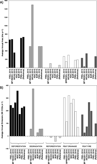
Figure 2. Reported estimates of (a) the area impacted by each activity, and (b) emissions due to each activity, from each government-led inventory and our reference estimate. Inventories that report emissions from, but not the area impacted by, a given activity are blank in (a). Inventories that do not estimate emissions from an activity are blank in both (a) and (b).
Download figure:
Standard image High-resolution image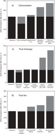
Figure 3. GHG fluxes from (a) deforestation, (b) peat drainage, and (c) peat fires, according to our reference approach, and each modification. The change relative to the reference is indicated by the grey portion of the bar.
Download figure:
Standard image High-resolution image
Additionally, the inventories largely base their calculations of GHG fluxes on the same carbon stock estimates from the National Forest Inventory (MoEF 2015a) (SI table 1). They also use the same Tier 1 estimates of emissions from peat drainage (SI table 2) and peat fire (IPCC 2013). The inventories that estimate emissions from below-ground biomass, necromass, and non-CO2 gases (SI table 3) use Tier 1 estimates (IPCC 2006a, 2006b, 2013). The exception is FREL 2014, which uses carbon stock data and peat emissions factor data based on the average of several national studies (SI tables 1 and 2). All the inventories assume that emissions from forest change and peat fires occur in the year of conversion (committed emissions), but assume that emissions from peat drainage occur in equal increments annually. The exception is INCAS 2015, which models GHG fluxes due to forest change over time.
3.2. Sensitivity assessment
Based on the reference approach, we estimated average annual GHG emissions of 0.47 Gt CO2e yr−1 over the 2000–2012 period, including 0.23 Gt CO2e yr−1 due to deforestation, 0.07 Gt CO2e yr−1 due to peat drainage, and 0.16 Gt CO2e yr−1 due to peat fires (figure 2(b)). Our reference emissions estimates fall within the range of the government-led inventories, except for our peat drainage estimate, which is lower. This may be because all reported peat drainage emissions estimates include at least one modification to the reference approach, such as the inclusion of methane emissions or legacy fluxes.
The largest changes to the reference deforestation GHG flux estimate occurred when we included emissions from belowground biomass and necromass pools (producing a 61% increase relative to reference), used alternative emissions factors (43% increase), and accounted for carbon sequestration due to forest regrowth after a deforestation event (31% decrease) (figure 3(a)). Including emissions due to plantation forest loss, which impacted an average of 62 kha yr−1, resulted in an increase of 7% relative to the reference.
Our reference peat drainage GHG flux estimate increased substantially when we included legacy emissions due to deforestation that occurred prior to the year 2000 (figure 3(b)). There are two ways that the inventories in this assessment account for legacy emissions: (1) all 5.8 Mha of non-forest peat lands in the year 2000 continue to emit GHGs due to a prior deforestation event, producing an estimate 151% higher than the reference, and (2) only the 2.6 Mha of peat lands that were deforested and drained over the period 1990–2000 continue to emit GHGs, producing an estimate 94% higher relative to the reference. Including non-CO2 emissions due to peat drainage, and using forest degradation as a proxy for peat drainage, increased emissions by just 4% each. When we used alternative emissions factors from the FREL 2014, our estimate of peat drainage emissions was 23% lower than the reference.
The largest changes to the reference peat fire GHG flux estimate resulted from modifying the assumptions of the mass of fuel burnt in a peat fire event (figure 3(c)). Increasing our estimate of the depth to which peat soils are burnt, and increasing the estimate of the bulk density of peat soils, resulted in emissions estimates which were 88% and 27% larger, respectively. When we accounted for methane emissions, our estimate of peat fire GHG emissions increased by 35% relative to the reference case. On the other hand, an average of just 19 kha of peat fires occurred in persistent forest lands each year, and therefore assuming these fires did not ignite peat soils reduced emissions by just 3% compared to the reference.
Our reference estimate of LULUCF emissions, of 0.47 Gt CO2e yr−1, almost doubled when we included all the modifications identified in our assessment, to 0.95 Gt CO2e yr−1. This difference is more than half of the observed 0.7 Gt CO2e yr−1 range between the lowest and highest inventory emissions estimates. The remaining disagreement can be explained in part by differences in input data, and resulting differences in estimates of the area impacted by each activity and emissions associated with each activity, and potentially by methodological differences that we were unable to identify in our review.
3.3. Synthesis
Differences in reported GHG fluxes over the study period are largely driven by varying degrees of inventory completeness, in terms of the scope of activities considered, the approach to define each activity, and the comprehensiveness of the GHG fluxes accounted for. The INCAS 2015 inventory is the most complete, because it incorporates fluxes from all activities, uses the broadest definition of each activity (e.g. includes peat fires even in persistent forests), and is the most comprehensive in accounting for component GHG fluxes (table 2). As a result, it reports the highest estimate of average GHG fluxes over the study period, of 1.1 Gt CO2e yr−1. The FREL 2014 inventory is intermediate in terms of completeness, as it excludes forest degradation and forest restoration activities, but accounts for fluxes from BGB and legacy emissions, resulting in an estimate of average GHG fluxes of 0.7 Gt CO2e yr−1. The FREL 2016 and BP REDD+ 2015 are the most conservative of the assessed inventories. The former does not consider peat fire activity, or non-CO2 gases and non-AGB pools, although it does account for legacy emissions from peat degradation, resulting in an estimate of average GHG fluxes of 0.5 Gt CO2e yr−1. On the other hand, BP REDD+ 2015 includes peat fire emissions and forest degradation emissions, but omits all other modifications described in table 2, resulting in the lowest average estimate of 0.4 Gt CO2e yr−1.
Unfortunately, the NDC submission (NDC 2015) and the recent biennial update report (BUR 2015) provide limited information on input data and methods. These inventories estimate GHG fluxes across all sectors of the economy, and do not therefore elaborate the LULUCF portion of the inventory to the same degree as the other inventories which focus specifically on LULUCF fluxes. The NDC 2015 inventory excludes forest degradation and forest restoration activities, but reports the highest emissions from deforestation and peat fires, possibly because of a relatively comprehensive treatment of all component GHG fluxes. On the other hand, BP REDD+ 2015 includes all five activities, but reports the lowest estimates of emissions from deforestation and forest degradation, possibly due to the omission of key GHG fluxes. As a result, the NDC 2015 inventory reports average GHG fluxes over the study period of 0.9 Gt CO2e yr−1, while the BP REDD+ 2015 inventory reports 0.6 Gt CO2e yr−1.
Although we focus on the underlying reasons for differences in average reported emissions over the 2000–2012 period, there are also clear differences in inter-annual variability reported by the studies (figure 1), driven by the inclusion of peat fire emissions. Peat fires correspond closely to differences in seasonal precipitation (Field et al 2009), and are therefore the most variable source of GHG emissions over time. The BUR 2015, INCAS 2015, and NDC 2015 inventories report similar temporal trends in emissions because they all estimate emissions from peat fires annually. This differs from FREL 2016, which does not consider peat fires, and BP REDD+ 2015, which estimates very small emissions from peat fires, and therefore report relatively stable emissions over the study period. The FREL 2014 reports peat fire emissions averaged over each three year period 2000–2012 and therefore reports a moderately variable trend.
4. Discussion
The challenges to constructing harmonized GHG inventories that we observe in Indonesia are likely to be faced by countries around the world, as they contend with the complexities of LULUCF GHG flux estimation across a range of purposes. Non-annex 1 countries recently committed to more regular GHG inventory reporting (UNFCCC 2012), have recently submitted NDCs, and may have submitted FRELs as the foundation for REDD+ performance tracking (UNFCCC 2014). Each policy purpose promotes a somewhat distinct approach to emissions estimation. For example, the REDD+ program encourages countries to submit conservative FRELs in order to avoid over crediting, which often results in the omission of fluxes which are not significant, have high uncertainty or have limited data availability (Grassi et al 2008). On the other hand, countries are encouraged to present complete GHG flux estimates in their biennial update reports. Although the UNFCCC Warsaw Framework for REDD+ instructs countries to maintain comparability among their FRELs and national GHG inventories (UNFCCC 2013), the Indonesia case demonstrates that there are several influential mythological differences across these inventory types.
It is expected that variations in LULUCF GHG inventory methods, assumptions, and definitions, driven by these diverse policy motivations, will result in different estimates of total GHG fluxes. In theory this may not be inherently problematic, as there are many acceptable methodological alternatives which necessarily produce different results. However, inconsistencies are problematic when direct comparisons among various inventories, or between national inventories and other emissions estimates, are needed. Typical comparisons include, for example, tracking emissions trends over time, or determining the contribution of a mitigation action to a national mitigation goal (Pelletier et al 2013). In addition, comparison between national and subnational inventories can be expected in the case of Indonesia, where 34 provincial governments are tasked with GHG flux accounting to support the development of local action plans reduce GHG emissions (Government of Indonesia 2011). Currently, comparability between national and subnational inventories is limited by similar issues identified in this assessment, including data discrepancies, variations in underlying methods, and lack of reporting transparency (Ge et al 2016).
We emphasize the following best practices to ensure that inventories can be appropriately compared, and make progress towards the IPCC principles of transparency, consistency, comparability, completeness, and accuracy (TCCCA).
4.1. Reporting framework detail
We observe that Indonesia's LULUCF GHG flux inventories frequently omit key methodological detail, and fail to disaggregate reported GHG fluxes by activity, land cover type, carbon pool, greenhouse gas, or legacy source. Providing separate estimates of component GHG fluxes will allow direct apples-to-apples comparison between inventories. For example, comparability would be substantially improved if all inventories separately reported estimates of gross CO2 emissions from AGB pools in the event of natural tree cover loss. Inventories which include additional fluxes, for example from BGB pools, methane fluxes, or legacy fluxes, should report these separately. This type of disaggregated reporting would support differentiation of disagreement produced by variations in estimation methods, from differences attributable to data uncertainties.
The IPCC guidance for national GHG inventories affords countries substantial methodological flexibility to account for a broad range of unique country circumstances. A clear requirement to ensure comparability is therefore a standardized reporting framework that facilitates clear articulation of underlying methods and assumptions, and separate reporting of partial fluxes (e.g. by activity, land cover type, carbon pool, greenhouse gas, or legacy source). The ongoing refinement of the 2006 IPCC guidelines for national GHG inventories is one opportunity to encourage enhanced reporting transparency, and specify appropriate levels of data aggregation (IPCC 2016). Another opportunity to encourage inventory harmonization and reporting detail is via the UNFCCC technical assessment process for FRELS, in which evaluators review and provide detailed feedback on submitted FRELs (UNFCCC 2014). This technical assessment process could include recommendations for countries with concurrent inventory efforts to identify underlying reasons for any observed differences.
4.2. Institutional coordination
In Indonesia, the merging of the Ministry of Environment with the Ministry of Forestry in 2015 consolidated jurisdiction over GHG inventory reporting and land cover monitoring and management (Muridyarso 2014). However, this consolidation did not immediately clarify roles and responsibilities for LULUCF GHG inventory tasks: since 2014 at least four agencies and directorates reported different LULUCF GHG flux estimates at the national level (table 1). This shifting authority resulted in divergent methodologies and inefficiencies, as data collection, management, and reporting systems were rebuilt. A priority for harmonizing LULUCF GHG inventories is therefore a dedicated and permanent institution mandated with data collection, synthesis and reporting. Such an institution could also set nationally appropriate methodological standards for subnational GHG inventories, calculation of mitigation impacts, and recalculation of GHG flux estimates using newly available data, to ensure comparability and time series consistency. The nation's SIGN SMART system for GHG inventories is one tool that is currently operational, and has the potential to facilitate further institutional coordination.
4.3. Input data improvement
A recent global assessment of national GHG inventories found that the omission of uncertain GHG fluxes, including from forest degradation and forest regrowth, from belowground and necromass pools, and of non CO2 gases, is commonplace (Federici et al 2017). Indeed, several of the inventories assessed in this study, particularly those designed for FREL development, mention data uncertainty as the reason for excluding a flux component (although none specify the magnitude of uncertainty of these fluxes). Specifically, the FREL 2014 and the FREL 2016 omit GHG fluxes from an entire class of activity (forest degradation and peat fires, respectively) and non-CO2 greenhouse gases, and BP REDD+ 2015 and FREL 2016 omit all carbon pools except for AGB. In the near term, completeness can be improved by including default (Tier 1) emissions factors until more detailed country-specific (Tier 2) estimates, or locally parameterized emissions models (Tier 3), are available (IPCC 2006a). In principle, GHG flux estimates should be consistent regardless of the data tier, but with larger uncertainty bounds for Tier 1 data than for Tier 3 data.
Over a longer time frame, an important strategy for encouraging inventory completeness is to increase confidence in estimates of GHG fluxes from key sources, by expanding the scope of data collection efforts. Others have noted the importance of improving the accuracy of estimates of LULUCF activity and emissions factor data across the tropics, and of peat land extent and peat carbon content specifically in Indonesia (e.g. Warren et al 2017). There is substantial ongoing research focused on estimating key GHG fluxes in Indonesia, including projects aimed at improving the accuracy of peat land extent and depth measurements (WRI 2018). This study highlights several additional research priorities, including estimation of GHG fluxes from belowground biomass and necromass pools, long term emissions due to peat drainage, the extent of peat drainage and peat fires, and the mass of fuel burnt in a peat fire event.
4.4. Comprehensive uncertainty assessment
Only two of the six inventories report uncertainty; INCAS 2015 estimates uncertainty of deforestation emissions, but does not report a resulting confidence interval, while FREL 2016 estimates average uncertainty of ±16.1% from all activities. A priority for future inventories in Indonesia will be more systematic and comprehensive estimation of uncertainty, by propagating the uncertainty distributions for all input parameters through the inventory model (Griscom et al 2016). In addition to providing a gauge of the reliability of GHG inventories in general, clearly articulated uncertainty estimates are pre-requisite for identifying inventory components which should be priority targets for future scientific inquiry, underpinning confidence intervals for future emissions projections, determining conservative estimates of the success of mitigation actions (Grassi et al 2008), and potentially informing approaches for adjusting results-based payments for emissions reductions (Pelletier et al 2015).
This study highlights that a critical step for uncertainty assessments will be to isolate uncertainties associated with input data from differences due to alternative inventory model specifications, definitions, and assumptions. Using Panama as a case study, Pelletier et al 2013 demonstrated a method for doing this, by incorporating alternative inventory model assumptions into a Monte Carlo uncertainty assessment via binary inclusion/exclusion (Pelletier et al 2013). Given the magnitude of disagreement produced by alternative approaches observed in the present study, a similar approach to uncertainty quantification that enables comparison of uncertainty driven by input data versus model specification may be valuable in the context of Indonesia.
5. Conclusion
The Indonesian government's success in achieving its climate change mitigation goal will depend on its ability to measure progress and evaluate the effectiveness of abatement actions, for which reliable GHG inventories are an essential foundation. There is currently a large range in LULUCF GHG flux estimates among inventories, on par with the magnitude of Indonesia's GHG emissions mitigation target. We observe that these differences are driven by variations in input data, methods, assumptions, and definitions, that collectively contribute more than half of observed discrepancies among inventory estimates. Direct comparison among GHG flux estimates constructed using different approaches is inappropriate, as it could potentially lead to biased conclusions concerning, for example, the magnitude of GHG emissions reductions, or emissions trends over time. In addition to ongoing efforts to reduce input data uncertainties, a priority for future GHG inventories will therefore be more transparent and detailed reporting. This recommendation is also relevant in other country contexts, as nations face the challenge of harmonizing LULUCF GHG flux estimates to support a range of policy instruments including NDCs and REDD+.
Acknowledgments
We thank two anonymous reviewers for their helpful feedback on earlier versions of this manuscript. This research was developed at the Center for International Forestry Research and Bogor Agricultural University, with financial support from the Fulbright US Scholar Program. KGA is supported by the National Science Foundation's Graduate Research Fellowship Program (DGE-1106401). The funders had no role in study design, data collection and analysis, decision to publish, or preparation of the manuscript.