


Abstract
We estimate the technical potential of rooftop solar photovoltaics (PV) for select US cities by combining light detection and ranging (lidar) data, a validated analytical method for determining rooftop PV suitability employing geographic information systems, and modeling of PV electricity generation. We find that rooftop PV's ability to meet estimated city electricity consumption varies widely—from meeting 16% of annual consumption (in Washington, DC) to meeting 88% (in Mission Viejo, CA). Important drivers include average rooftop suitability, household footprint/per-capita roof space, the quality of the solar resource, and the city's estimated electricity consumption. In addition to city-wide results, we also estimate the ability of aggregations of households to offset their electricity consumption with PV. In a companion article, we will use statistical modeling to extend our results and estimate national rooftop PV technical potential. In addition, our publically available data and methods may help policy makers, utilities, researchers, and others perform customized analyses to meet their specific needs.
Export citation and abstract BibTeX RIS
1. Introduction
How much energy could be generated by select US cities if solar photovoltaic (PV) systems were installed on all their suitable roof area? This quantity is the technical potential of rooftop PV for those cities—an established reference point for renewable technologies that quantifies the generation available from a particular resource (e.g. see Lopez et al 2012). The metric considers the resource's availability and quality, the performance of the technology capturing the resource, and the physical area suitable for development. It does not consider economics, growth potential, or grid-integration factors, and thus it is an upper limit of a technology's current potential generation, not a prediction of expected deployment.
In this article, we estimate the technical potential of PV systems on existing suitable roof area in select US cities. To produce this estimate, the fraction of rooftop area suitable for PV must be estimated. Melius et al (2013) identify three main approaches to estimating rooftop suitability: constant-value methods, manual selection, and methods based on geographic information systems (GIS). Constant-value methods assume a certain percentage of building rooftop area is suitable for hosting PV and then applies these percentages to the total building stock to estimate the area available for PV; most previous estimates of national PV technical potential have relied on such methods (e.g. Chaudhari et al 2004, Denholm and Margolis 2008, Frantzis et al 2007, Paidipati et al 2008). This method is simple and quick, but it often has had little validation and does not consider the nuances of individual buildings. In contrast, manual selection evaluates the suitability of individual buildings using sources such as aerial photography, Google Earth, and the National Renewable Energy Laboratory's PVWatts® Calculator to provide visual clues to PV installation locations (Ordonez et al 2010, Bright and Burman 2010, Zhang et al 2009, Anderson et al 2010). Manual selection is precise but time consuming, and it cannot be replicated easily on a large scale. GIS-based methods provide more precision than constant-value methods while handling much larger data sets than manual selection. Melius et al (2013) give many examples of GIS-based applications (e.g. Hofierka and Kanuk 2009, Compagnon 2004, Santos et al 2011), and they develop and validate a suitability-estimation method based on best practices from the literature.
We use the validated GIS-based method from Melius et al (2013) to provide a detailed data-driven analysis of US rooftop PV suitability and technical electricity-generation potential. Specifically, we use light detection and ranging (lidar) data, GIS methods, and PV-generation modeling to calculate the PV suitability of rooftops for 128 cities nationwide—representing approximately 23% of US buildings—and we provide PV-generation results for a subset of these cities. In a subsequent Environmental Research Letters article, we will use statistical modeling to extend these results and estimate national rooftop PV technical potential2.
2. Methods
Figure 1 summarizes our method for estimating rooftop PV suitability. Inputs include lidar and building footprint data sets. These data are processed to determine the shading, tilt, and azimuth of each rooftop at a horizontal resolution of 1 m2. A set of criteria is then applied to determine what roof area is suitable for PV deployment. These results can then be aggregated to determine the total quantity of rooftop area suitable for PV systems at various scales. Once the suitable rooftop area is quantified, the potential PV electricity generation is calculated.
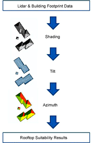
Figure 1 Major steps for determining the suitability of roof area for PV.
Download figure:
Standard image High-resolution imageMelius et al (2013) validate this rooftop suitability estimation method against installation data from 205 PV arrays across three states. They show that 89% of modeled slopes were within 10 degrees of the actual slope, 99% of modeled orientations matched the actual orientations, and 99% of modeled results had the actual required minimum number of sun hours for PV to produce 80% generation. All arrays used in the validation process showed at least some of the rooftop was suitable for PV, and 79% had an area at least the size of the actual installed system.
2.1. Input data
Our lidar data were obtained from the US Department of Homeland Security (DHS) Homeland Security Infrastructure Program for 2006–2014. For each of the 128 cities in the data set, DHS provided (1) lidar data in raster format at 1 m by 1 m resolution and (2) a corresponding polygon shapefile of building footprints. The raster data are based on the reflective surface return (first return) of the lidar data, which correlates to the elevation of the first object detected and creates a digital surface model for each city.
The DHS data set also includes detailed data for about 26.9 million buildings and 7.7 billion m2 of rooftop area, or about 23% of US buildings (EIA 2009, EIA 2012). The area covered (figure 2) represents about 122 million people or 40% of the US population. To better understand the suitability and technical potential of buildings of various sizes, we subdivided all buildings into three classes according to the planar area of their footprints:
- Small: < 5000 ft2 (94% of buildings, 58% of rooftop area in our sample).
- Medium: 5000–25 000 ft2 (5% of buildings, 18% of rooftop area in our sample).
- Large: > 25 000 ft2 (1% of buildings, 24% of rooftop area in our sample).
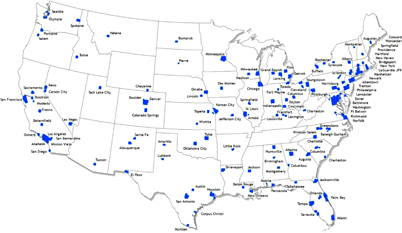
Figure 2 Lidar data coverage.
Download figure:
Standard image High-resolution image2.2. Shading
Our first step in processing the lidar data was to run a shading simulation on the digital surface model of each city3. Figure 3 provides an example simulation output, showing how the shadows move throughout a single day. Seasonal variation in shading was captured by running the simulation for four days: March 21, June 21, September 21, and December 21. The hours of sunlight each square meter received for the four days were averaged to determine an average number of hours of daily sunlight for each square meter, as shown in figure 4 4.

Figure 3 Example of hourly shading and sunlight availability.
Download figure:
Standard image High-resolution image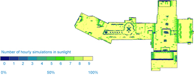
Figure 4 Example of average daily hours of sunlight.
Download figure:
Standard image High-resolution image2.3. Orientation (tilt and azimuth)
We determined the tilt for each square meter of roof area within our lidar data set. To be consistent with many roofers' and PV installers' definition of flat roofs, we defined all roof area with a tilt less than 9.5 degrees as 'flat.' Because illumination is calculated by the angle at which the sun hits a surface, the shading simulation underestimates sun exposure for these flat roofs. For a subset of flat roof areas, we quantified the difference between predicted hours of sunlight and actual hours derived from installed system data. Applying a multiplier of 1.5 to the predicted illumination of all flat roofs compensated for this difference.
We also determined the azimuth for each square meter of roof area. Each square meter was categorized into one of nine azimuth classes (figure 5), where tilted roof areas were assigned one of the eight cardinal and primary intercardinal directions; area with a tilt less than 9.5 degrees was classified as flat. As described in section 2.4, the northwest, north, and northeast azimuths were defined as unsuitable, resulting in five non-flat azimuth classes and one flat class.

Figure 5 Nine azimuth classifications.
Download figure:
Standard image High-resolution imageThe azimuth file was then run through a variety function, which returned the number of different values in the 3 × 3 neighborhood surrounding each square meter of roof area. Area bordered by more than three unique azimuths was excluded from the data set to remove areas of changing roof orientations and excessively noisy data.
We then used the azimuth values to identify roof planes by assuming contiguous areas of identical azimuth class were a unique plane, and we aggregated each of the individual square meters of roof area into polygons representing contiguous roof planes. For each of the individual roof planes, the ArcGIS Zonal Mean tool was applied to the tilt raster to determine the roof plane's mean tilt. The data set produced through this process consisted of a raster giving a single tilt value for each unique roof plane.
Once the individual square meters of roof area were aggregated into contiguous planes, we categorized each plane into one of 21 orientation classes based on its tilt and azimuth, defining a set of four tilt classes (figure 6), the aforementioned five azimuth classes, and a 'flat' class. These classes were then used in the PV electricity generation modeling process (section 2.5) to more accurately estimate the productivity of each roof plane.
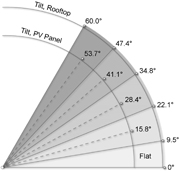
Figure 6 Tilt classes.
Download figure:
Standard image High-resolution image2.4. Application of suitability criteria
To determine the total roof area suitable for PV, we excluded area that did not meet criteria for shading, tilt, azimuth, and a minimum amount of contiguous roof area. For each city, we used the System Advisor Model (SAM) to calculate the number of hours a rooftop would need to be in sunlight to produce 80% of the energy produced by an unshaded system of the same orientation. Roof area that did not meet this shading criterion was excluded based on input from solar installers and research analysts, who suggested this minimum threshold was toward the low end of best practices (i.e. installing a system that received more shade would not generally be recommended).
Roof planes were also excluded based on their orientation. All roof planes facing northwest through northeast (292.5–67.5 degrees) were considered unsuitable for PV and excluded owing to a lack of direct sunlight. All tilt values greater than 60 degrees were removed from the data set, based on the recommendation of PV installers; in any case, our data show that roof planes of 60 degrees or steeper are very uncommon compared with more gradual planes.
We also required a PV-suitable roof to have at least one contiguous plane with a projected horizontal footprint of 10 m2 or greater that also meets the shading, tilt, and azimuth criteria5. Doing so provides sufficient area to install a 1.6 kW system, assuming a 16%-efficient panel. We selected this minimum size threshold to represent a conservative lower-end estimate of viable PV system sizes, based on current PV performance and historical patterns in reported PV system sizing. Specifically, we reviewed reported system sizes for small PV systems (< 10 kW) through 2014 (Barbose and Darghouth 2015) and determined that 96% of systems in this class were larger than 1.6 kW. We considered a higher threshold of 3 kW, but 20% of historical sub-10 kW systems would not have exceeded this value, and therefore we considered it too high.
We calculated the area of each suitable roof plane, both as a projected area consistent with the building footprint and as a tilted area, to determine the actual amount of developable area. Ultimately, we used the tilted-area values to calculate the installed PV capacity.
The final data set contains the suitable area of every roof plane in the 128 cities covered by lidar data. This data set can be aggregated to the level of a building, ZIP code, utility service territory, state, or any other region to develop summary statistics describing the suitability of the geographic region for rooftop PV.
2.5. Simulation of PV productivity on suitable rooftop area
Our next step was to simulate the productivity of PV modules covering the suitable roof area within the 21 different orientation bins for every ZIP code in the lidar data set. These PV performance simulations were executed using SAM (version 2015.1.30). SAM is a performance and economic model designed to facilitate decision making and analysis for renewable energy projects (Gilman and Dobos 2012). It uses hourly meteorological data, a PV performance model, and user-defined assumptions to simulate the technical performance of a PV installation.
The solar resource and meteorological data used for this analysis are from the Typical Meteorological Year 3 (TMY3) data set of the National Solar Radiation Database (Wilcox and Marion 2008). The TMY3 data set includes hourly representative profiles for 1001 stations throughout the United States. For a given simulation, we used the TMY3 station profile closest to the boundary of the ZIP code under consideration. Because the TMY3 stations are frequently located in or near major cities, the average distance from a ZIP code to a station for the lidar data set was 9 km.
The technical performance of PV systems can also vary depending on the equipment used and design choices of the installer. We made a set of technical assumptions to represent the average performance of PV systems as they are being installed in 2015 (table 1). We used these values in SAM, in conjunction with the TMY3 solar resource and meteorological profiles, to determine the electrical output of PV systems6.
Table 1. Assumptions for PV Performance Simulations.
| PV System characteristics | Value for flat roofs | Value for tilted roofs |
|---|---|---|
| Tilt | 15 degrees | Midpoint of tilt class (figure 6) |
| Ratio of module area to roof area | 0.70 | 0.98 |
| Azimuth | 180 degrees (south facing) | Midpoint of azimuth class |
| Module power density | 160 W m−2 | |
| Total system losses | 14.08% | |
| Inverter efficiency | 96% | |
| DC-to-AC ratioa | 1.2 | |
aA system's direct current to alternating current (DC-to-AC) ratio is the ratio of the nameplate capacity of the PV modules to the AC-rated capacity of the inverters. For example, a system with a DC-to-AC ratio of 1.2 would have 8.33 kW of inverters installed for every 10 kW of nameplate PV capacity.
The power density value used in this analysis corresponds to a module with approximately 16% efficiency. This value is the median module efficiency from approximately 48000 systems installed during 2014 (Barbose and Darghouth 2015). This value was selected to represent an installed mixture of monocrystalline-silicon, multicrystalline-silicon, and thin-film modules, as opposed to universal installation of premium systems.
The losses from soiling, shading, snow, wiring, and other sources are captured in the total system losses parameter, which was chosen to remain at the SAM default value for this analysis. The inverter efficiency value also remained at the SAM default level. These levels have been selected to be representative of typical systems. A DC-to-AC ratio of 1.2 was selected based on existing literature on the optimal sizing of inverters to minimize the cost of PV-generated electricity (Mondol et al 2009).
For flat roofs, the ratio of module area to roof area was assumed to be 0.7 to reflect the row spacing necessary to incur only approximately 2.5% losses from self-shading for south-facing modules at 15-degree tilt. For tilted roofs, the value was assumed to be 0.98 to reflect 1.27 cm of spacing between each module for racking clamps7.
Using the above assumptions, we ran simulations in SAM to estimate the installed capacity and annual energy generation for each roof plane. We modeled all planes assuming a PV system aligned with the midpoint values of their orientation class' tilt and azimuth ranges. For example, any roof plane with a tilt value between 47.4 and 60.0 degrees and an azimuth between 157.5 and 202.5 degrees was modeled with a module tilted at 53.7 degrees and facing 180 degrees (south). We then summed the potentials of all of the roof planes within a ZIP code to arrive at total production values.
3. Results and discussion
Small buildings—with their more diverse architectures and more shadowing from trees and neighboring buildings—show substantially more variability in rooftop PV suitability than do medium and large buildings (table 2). Within the 128 cities covered by our lidar data, 83% of small buildings have a suitable PV installation location, but only 26% of the total rooftop area of small buildings is suitable for development8. There is some variability among states, with central and southeastern states showing the greatest fraction of suitable rooftops on small buildings. In contrast, more than 99% of large and medium buildings have at least one qualifying roof plane, with 49% of total rooftop area suitable for medium buildings and 66% for large buildings. Across all building sizes, 32% of total rooftop area is suitable for PV deployment.
Table 2. Roof Area Suitability Trends by Building Class.
| Building Class (Building Footprint) | Percent of Buildings with a Suitable Location | Percent of Total Area that is Suitable |
|---|---|---|
| Small (< 5000 ft2) | 83% | 26% |
| Medium (5000–25 000 ft2) | 99% | 49% |
| Large (> 25 000 ft2) | 99% | 66% |
| All Buildings | 84% | 32% |
Flat planes are very common on large buildings (93% of planes on large buildings are flat) and medium buildings (74%) but less common on small buildings (26%). Most other suitable rooftop planes fall into the 28 degree tilt category, and steep rooftops (54 degrees) are an order of magnitude less common than the next category (41 degrees). Azimuths facing east, west, and south are most common, particularly among the 28 degree category of rooftops. These azimuths correspond to the alignment of buildings on a cardinal street grid. These observations appear to hold for small, medium, and large buildings alike. Large cities have the most flat-roofed small buildings, with the fraction decreasing in more urbanized areas. Large cities also have a more homogeneous tilt/azimuth distribution than do small suburbs.
The following subsections provide detailed suitable-rooftop-area and PV-generation results for select cities.
3.1. Small buildings
We mapped results for 11 cities chosen based on (1) good coverage of the ZIP codes within each city's boundaries and (2) how the cities illustrate the data variation geographically. Figure 7 shows the percentage of small buildings that have at least one suitable roof plane at the ZIP-code level. Only the suitability of small buildings is mapped, because over 99% of medium and large buildings have at least one roof plane suitable for PV deployment. Figure 7 and figure 8 both show the nominal city boundaries, as defined by the US Census Bureau 2013 TIGER/Line Shapefiles.
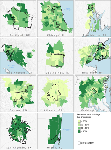
Figure 7 Percent of small buildings with at least one plane suitable for PV by ZIP code in 11 select cities.
Download figure:
Standard image High-resolution image
Figure 8 Small building average relative production for 11 select cities (average small building PV production / state average household electricity consumption).
Download figure:
Standard image High-resolution image
Figure 7 shows only a weak trend of high building density driving down the suitability of small buildings. Most of the highly developed downtown ZIP codes in the 11 cities have suitability similar to the suitability in other ZIP codes within the city boundaries, although some suburban ZIP codes outside city boundaries show higher levels of suitability.
Figure 8 shows the average relative production of small buildings, which is defined here as the annual electricity generation potential for an average small building as a percentage of the average household annual electricity consumption in that city's state (EIA 2009). Because the national building stock is estimated to contain 78 million single-family households but only 3.2 million commercial buildings with a footprint less than 5000 ft2, figure 8 can be interpreted as approximately comparing the potential electricity production of an average single-family household in a given ZIP code with the state average household electricity consumption9. This metric should not be confused with the ability of small-building PV to offset a state's total electricity sales. Furthermore, because this metric includes buildings unsuitable for PV and presents an average for each ZIP code, it should not be interpreted as predicting the productivity of individual buildings, which would vary significantly within each ZIP code.
Figure 8 shows strong regional variation in the average relative production of small buildings. The average productivity of households within a ZIP code is driven by average suitability, household footprint, and solar resource. The average relative production is then also a function of the state average household consumption. For example, high-quality solar resource and low state average household energy consumption lead to a high average relative production for small buildings in Los Angeles. However, the outcome of the interaction among these four drivers is not always obvious. For example, although Colorado has low state average household consumption (7.4 MWh/year or 65% of the national average), Denver's low suitability, moderate solar resource, and moderate household sizes lead to generally low average relative production for small buildings within the city boundaries. In contrast, despite Florida's relatively high state average household consumption of 14.8 MWh/year (130% of the national average) and low state average square footage per housing unit (85% of the national average), Miami's high suitability and good solar resource result in generally high average relative production for small buildings. This demonstrates that one or even two metrics are not sufficient for predicting the ability of aggregations of households to offset their consumption.
Although it is generally understood that a household with adequate roof area can generate greater than 100% of its annual energy consumption with PV, the variation in rooftop suitability and building characteristics makes it less obvious whether that trend holds for groups of buildings. This analysis suggests that, in many parts of the United States, ZIP-code-sized aggregations of households can collectively generate an amount of electricity that exceeds their annual consumption. However, notable exceptions include Atlanta and Portland, which have relatively few ZIP codes in which annual energy generation would match expected consumption as estimated by state average household consumption.
3.2. All buildings
To summarize the technical potential of the lidar regions at an accessible resolution, we aggregated the ZIP code results for 47 cities whose ZIP codes all have at least some coverage by the DHS lidar data and have ZIP code boundaries that approximately align with city boundaries (US Census Bureau 2013 TIGER/Line Shapefiles). In contrast to the previous section, which only explored data for small buildings, the results here aggregate the productivity of all building sizes. Table 3 gives the estimated total installed capacity and annual energy generation potential for the 47 cities. Many cities have lidar data that extend beyond official city boundaries. ZIP codes outside the city boundaries were not included in calculations of the total capacity and energy estimates.
Table 3. Technical Potential of Rooftop PV from all Building Sizes within Boundaries of Cities Completely Covered by lidar Data.
| City | Installed Capacity Potential (GW) | Annual Generation Potential (GWh/year) | Ability of PV to meet Estimated Consumption |
|---|---|---|---|
| Mission Viejo, CA | 0.4 | 587 | 88% |
| Concord, NH | 0.2 | 194 | 72% |
| Sacramento, CA | 1.5 | 2293 | 71% |
| Buffalo, NY | 1.2 | 1399 | 68% |
| Columbus, GA | 1.1 | 1465 | 62% |
| Los Angeles, CA | 9.0 | 13 782 | 60% |
| Tulsa, OK | 2.6 | 3590 | 59% |
| Tampa, FL | 1.4 | 1952 | 59% |
| Syracuse, NY | 0.6 | 657 | 57% |
| Amarillo, TX | 0.7 | 1084 | 54% |
| Charlotte, NC | 2.6 | 3466 | 54% |
| Colorado Springs, CO | 1.2 | 1862 | 53% |
| Denver, CO | 2.3 | 3271 | 52% |
| Carson City, NV | 0.2 | 386 | 51% |
| San Antonio, TX | 6.2 | 8665 | 51% |
| San Francisco, CA | 1.8 | 2684 | 50% |
| Little Rock, AR | 0.8 | 1099 | 47% |
| Miami, FL | 1.4 | 1959 | 46% |
| Birmingham, AL | 0.9 | 1187 | 46% |
| St. Louis, MO | 1.5 | 1922 | 45% |
| Cleveland, OH | 1.7 | 1881 | 44% |
| Toledo, OH | 1.4 | 1666 | 43% |
| Providence, RI | 0.5 | 604 | 42% |
| Worcester, MA | 0.5 | 643 | 42% |
| Atlanta, GA | 1.7 | 2129 | 41% |
| New Orleans, LA | 2.1 | 2425 | 39% |
| Hartford, CT | 0.4 | 404 | 38% |
| Baltimore, MD | 2.0 | 2549 | 38% |
| Bridgeport, CT | 0.4 | 435 | 38% |
| Detroit, MI | 2.6 | 2910 | 38% |
| Portland, OR | 2.6 | 2811 | 38% |
| Milwaukee, WI | 2.1 | 2597 | 38% |
| Boise, ID | 0.5 | 760 | 38% |
| Des Moines, IA | 0.8 | 1026 | 36% |
| Cincinnati, OH | 1.0 | 1176 | 35% |
| Norfolk, VA | 0.8 | 1047 | 35% |
| Wichita, KS | 1.1 | 1537 | 35% |
| Newark, NJ | 0.6 | 764 | 33% |
| Philadelphia, PA | 4.3 | 5289 | 30% |
| Springfield, MA | 0.3 | 370 | 29% |
| Chicago, IL | 6.9 | 8297 | 29% |
| St. Paul, MN | 0.8 | 903 | 27% |
| Pittsburgh, PA | 0.9 | 907 | 27% |
| Minneapolis, MN | 1.0 | 1246 | 26% |
| Charleston, SC | 0.3 | 407 | 25% |
| New York, NY | 8.6 | 10 742 | 18% |
| Washington, DC | 1.3 | 1660 | 16% |
To enable a simple estimation of these cities' abilities to offset their electricity consumption with PV, each state's total electric-industry sales were distributed to its cities by population weight. For example, Florida has 222 TWh of annual sales, and 1.5% of Florida's population lives within the boundaries of Tampa; therefore, the estimated consumption of Tampa is 3.33 TWh. This approximation will overestimate the potential for PV to meet a city's actual consumption for cities that consume more per capita than the state average, and it will underestimate the potential for cities that consume less.
Owing to their size and building density, the cities with the largest potential installed capacity are Los Angeles and New York, with 9.0 GW and 8.6 GW, respectively—illustrating that, even in dense urban areas, shading from buildings does not prevent appreciable PV installation. Even with large potential capacities in these dense cities, however, PV cannot meet the same percentage of city electricity demand as can be met in some smaller cities. For example, Syracuse and New York City have similar solar resources, but Syracuse can generate 57% of its associated consumption with rooftop PV, whereas New York City can generate only 18%. The total percentage of roof area suitable for PV is similar in the two cities (48% in Syracuse and 46% in New York City), suggesting the difference is driven by low roof area per capita in New York City.
Mission Viejo has relatively high per capita production, driven in part by a low proportion of multi-unit households (which constitute only 15% of total housing units, as compared to an average of 30% throughout the rest of California), resulting in a high quantity of residential roof area per resident. When combined with a relatively low average state per capita consumption and high-quality solar resource, the city can generate 88% of its estimated consumption using rooftop PV.
4. Conclusion
Based on our analysis of cities completely covered by lidar data, rooftop PV's ability to meet estimated electricity demand varies widely—from meeting 16% of demand (in Washington, DC) to meeting 88% (in Mission Viejo, CA). Important drivers include average rooftop suitability, household footprint/per-capita roof space, and solar resource as well as estimated electricity consumption. All these metrics must be considered in order to predict the ability of aggregations of households to offset consumption with rooftop PV.
Our results require several caveats. First, they are sensitive to assumptions about PV system performance, which is expected to continue improving. For example, if we assumed an average module efficiency of 20% instead of 16%, each technical potential estimate would increase by about 25%. Second, we only estimate the potential from existing, suitable roof planes—not the immense potential of ground-mounted PV. Actual generation from PV in urban areas also could exceed these estimates if systems were installed on less suitable roof area, PV were mounted on canopies over open spaces such as parking lots, or PV were integrated into building facades. Finally, our results do not consider the full set of challenges related to exploiting PV's technical potential. In practice, integrating significant rooftop PV into the national electricity portfolio would require a more flexible grid, supporting infrastructure, and a suite of enabling technologies.
The results we present here provide valuable insights into the technical potential of US rooftop PV, and—in a subsequent Environmental Research Letters article—we will use statistical modeling to extend these results to a nationwide estimate of technical potential. Just as importantly, we hope our data and methods spur creative future analyses by municipalities, utility providers, solar energy researchers, and others. We have made a wide range of data from our analysis publically available, including regional and ZIP-code-level summaries for all areas with lidar data10.
Acknowledgments
This work was funded by the Solar Energy Technologies Office of the US Department of Energy's Office of Energy Efficiency and Renewable Energy under contract number DE-AC36-08GO28308. The authors would like to thank Mike Gleason, Carolyn Davidson, Sean Ong, Rebecca Hott, Steve Wade, Eric Boedecker, Paul Denholm, Donna Heimiller, Michael Bolen, Laura Vimmerstedt, and Paul Donohoo-Vallett for their reviews and input. We would like to thank Adnan Zahoor, Britney Sutcliffe, and Julian Abbott-Whitley for their assistance in processing data. Lastly, we would like to thank Jarett Zuboy for his diligence and attention to detail while editing this article.
Footnotes
- 2
Additional detail on the method and results is provided in Gagnon et al (2016).
- 3
The standard ArcGIS Hillshade tool (available in the Spatial Analyst extension, ESRI 2014) was used for the shading simulation.
- 4
For each month, we determined a different threshold of illumination required to classify a cell as being in sunlight; March requires 60% illumination (values > 152), June 70% (values > 178), September 60% (values > 152), and December 50% (values > 127).
- 5
Only about 7% of sampled roof planes are smaller than 10 m2.
- 6
Documentation of the mathematical models used by SAM can be found internally within the program, under the 'Help' Section (see sam.nrel.gov).
- 7
Representative spacing between modules for racking clamps was obtained from a SnapNrack Series 100 UL installation manual, a SunFix Plus Installation Guide, and an IronRidge Roof Mountain System Design Guide. These racking systems are meant to illustrate existing products; mentioning them does not constitute an endorsement.
- 8
Because of obstructions, the tilt of a small fraction of roof area within the lidar data set was unknown. Statements about the total percentage of suitable roof area therefore assume the obstructed rooftops follow the same distribution of tilt as the rest of the stock.
- 9
Because the consumption value is a state average, it is constant across all ZIP codes for a given city and therefore does not capture household-level variation in consumption that would be driven by socioeconomic status, building size, or other household-specific factors. Therefore, the average relative production value mapped in figure 8 should only be interpreted as a simple estimation of the potential ability for a group of households in a given ZIP code to offset its consumption.
- 10
See maps.nrel.gov/pv-rooftop-lidar. Detailed documentation of each step in our analysis, including scripts for running the GIS tools, are linked to in the metadata section of each layer. This information can be accessed by clicking the question mark icon next to each layer in the table of contents in the Data Viewer.