

Abstract
It is well known that short-term (i.e. interannual) variations in fossil-fuel CO2 emissions are closely related to the evolution of the national economies. Nevertheless, a fraction of the CO2 emissions are linked to domestic and business heating and cooling, which can be expected to be related to the meteorology, independently of the economy. Here, we analyse whether the signature of the inter-annual temperature anomalies is discernible in the time series of CO2 emissions at the country scale. Our analysis shows that, for many countries, there is a clear positive correlation between a heating-degree-person index and the component of the CO2 emissions that is not explained by the economy as quantified by the gross domestic product (GDP). Similarly, several countries show a positive correlation between a cooling-degree-person (CDP) index and CO2 emissions. The slope of the linear relationship for heating is on the order of 0.5–1 kg CO2 (degree-day-person)−1 but with significant country-to-country variations. A similar relationship for cooling shows even greater diversity. We further show that the inter-annual climate anomalies have a small but significant impact on the annual growth rate of CO2 emissions, both at the national and global scale. Such a meteorological effect was a significant contribution to the rather small and unexpected global emission growth rate in 2014 while its contribution to the near zero emission growth in 2015 was insignificant.
Export citation and abstract BibTeX RIS

Original content from this work may be used under the terms of the Creative Commons Attribution 3.0 licence.
Any further distribution of this work must maintain attribution to the author(s) and the title of the work, journal citation and DOI.
1. Introduction
Scientists and policymakers pay attention to the evolution of energy related carbon dioxide (CO2) emissions as the main driver for present and future climate change. CO2 emissions from fossil fuels and industry, as reported by Olivier et al (2015) and Le Quéré et al (2016) grew by approximately 0.5% between 2013 and 2014 and stalled in 2015. The fairly small increase in 2014 despite continued economic growth came as a surprise for many stakeholders. Jackson et al (2015) cautiously suggested that this deceleration in CO2 emissions, which comes earlier than anticipated, may be the early sign of structural changes occurring in energy systems, in particular in China. However there could be other reasons for inter-annual variations in fossil-fuel CO2 emissions both at the national and global levels. For instance there could be small variations in CO2 emissions due to the year-to-year variations in the number of public holidays and a small increase can be expected on leap years, the latter effect being corrected in Le Quéré et al (2016). Meteorology is also known to affect energy consumption in many countries. While statistics for energy efficiency and final energy consumption are corrected for meteorological (e.g. mild winter) effects by some national statistics offices (e.g. in the UK and France), such corrections are not applied for energy consumption or for CO2 emissions reported in national inventories compiled and aggregated by international institutions (UNSD 2016, IEA 2016, UNFCCC, 2016). Considine (2000) showed that inter-annual weather variations have a sizeable (up to a few %) impact on carbon emissions in the United States. However this effect has not been quantified systematically and remains unknown for many countries. Although such an impact is likely to be small when aggregated at the global scale, it needs to be understood—and corrected for—if we want to interpret changes in CO2 emissions trends on the basis of a small number of years. In the following, we present our methodology and results on the signature of the inter-annual temperature anomalies in the time series of CO2 emissions at the country and global scales.
2. Data and method
2.1. CO2 emissions
We use estimates of national fossil fuel emissions of CO2 from EDGAR (European Commission, Joint Research Centre (JRC) and Netherlands Environmental Assessment Agency (PBL); version 4.3.2). This dataset provides yearly values of fossil fuel emissions from 1970 to 2015. CO2 emission estimates were made by PBL and the JRC on the basis of energy consumption data for the 1970–2013 period, published by the International Energy Agency (IEA, including the correction for China published in 2016), and on 2014–2015 trends, published by BP. The estimations are also based on production data on cement, lime, ammonia and steel developed jointly by the JRC and PBL (Olivier et al 2016). The time series of these emissions are shown for the 15 largest emitters in figure 1.
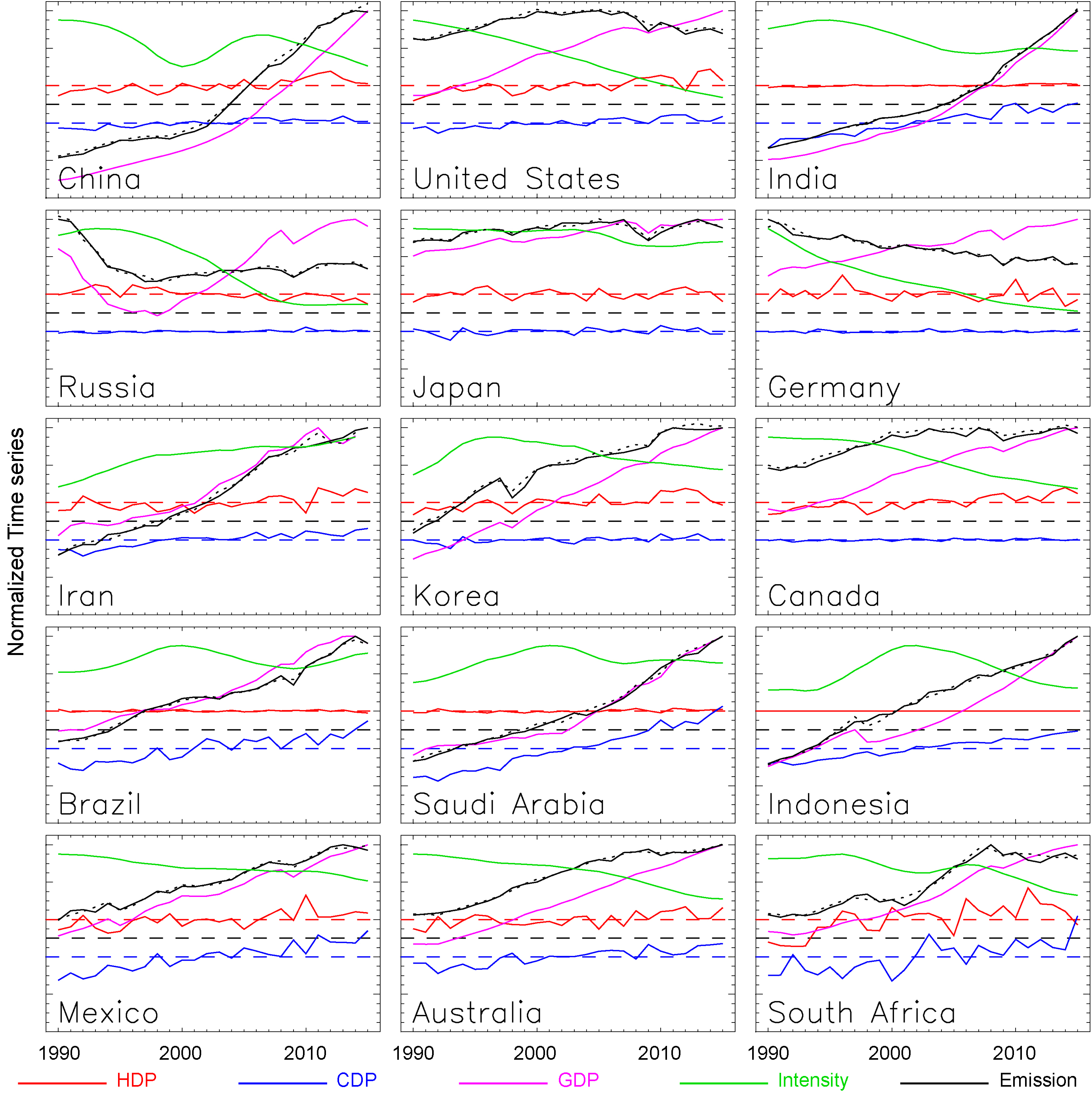
Figure 1 Time series of the variables that are used and derived from their analysis in this paper. This figure is for the 15 largest CO2 emitters as of 2014. A similar figure for the next 15 countries is provided in the supplementary material available at stacks.iop.org/ERL/12/074009/mmedia. For each subplot, the GDP, EMICO2 and intensity curves have been normalized to their maximal value. For the emission curve, the plain line is the actual estimate from EDGAR whereas the dotted line is the reconstructed value based on the GDP, CDP and HDP as per equation (1). The HDP and CDP curves have also been centered and normalized. The dashed line indicates the mean value and the scaling is such that the dashed black line indicates a 20% relative difference to the mean.
Download figure:
Standard image High-resolution image2.2. Economy
We use the gross domestic product (GDP) estimated by the World Bank (data.worldbank.org/indicator/NY.GDP.MKTP.KD/countries) as an indicator of the CO2 emissions that are directly related to variations in the national economies. These estimates are provided as constant 2010 US dollars and are available from 1960 to 2015 for 264 countries or group of countries. Although the time series have missing data for some countries, they are complete for the largest emitters that are of interest in this study.
Although the CO2 emissions depend on the GDP, one cannot assume that they are proportional. Indeed, numerous examples show that CO2 emissions do not increase as fast as GDP on the long term. This is due to improvement in the energy efficiency and the increasing share of the tertiary sector in the economy that produces less emission than the industrial sector for a given unit of GDP. We shall thus model CO2 emissions related to the economy as the product of the GDP and a slowly-varying intensity function Int(yr).
2.3. Meteorology
Heating and cooling are related to outside air temperature. Previous studies (e.g. Quayle and Diaz 1980 and references in Atallah et al 2015 and Azevedo et al 2015) have shown that heating is, to the first order, proportional to the temperature difference to a comfort temperature around 19 °C. Besides, considering only heating when the temperature is below a threshold further improves the correlation, at least in some cases such as for the gas consumption in the UK (Rahman 2011). The same has been observed for cooling (e.g Le Comte and Warren 1981 and references in Atallah et al 2015). The comfort and the threshold temperatures may vary. Here, we use 17 °C and 15 °C, so that we quantify heating-degree-day (HDD) as the sum over the year of the difference between 17 °C and the daily temperature whenever the daily temperature is lower than 15 °C, which corresponds to the expression applied by Eurostat (2010) for countries of the EU. We use a similar approach for the cooling (air conditioning) and the cooling-degree-day (CDD) is computed as the yearly sum of daily temperatures relative to 21 °C whenever they are greater than 24 °C. These thresholds can be considered as intermediate between those applied for Saudi Arabia and the United States, where references of 65 °F (≈18 °C) are used (Atallah et al 2015), and those deemed more realistic for China (Shi et al 2016), which only consider temperatures above 26 °C. The interested reader may refer to the abundant literature on the subject (e.g. Atallah et al 2015, Azevedo et al 2015, Isaac and van Vuuren 2009). Although different thresholds may be appropriate depending on the region, we make use of a single set for the whole world. As far as this study is concerned, we note that there is a robust basis in the literature to expect the HDD/CDD metrics to predict some amount of variance in CO2 emissions. As input meteorology data, we use the three-hourly ERA-interim reanalysis that is available from 1979 and updated in real time (Dee et al 2011) at a spatial resolution of ≈80 km (T255 spectral grid).
2.4. Population distribution
For the population distribution, we use the HYDE database, developed under the authority of the Netherlands Environmental Assessment Agency, that provides a time series of population and land use for the last 12 000 years at 5' resolution (Klein Goldewijk et al 2010). The dataset provides population maps for the years 1970, 1980, 1990, 2000 and 2005, which we interpolate linearly in time. Data from the SSP1 (Shared Socioeconomic Pathway 1; KC and Lutz 2017) scenario are used for 2005, 2010, 2015 and also interpolated in time.
2.5. Data processing
The HDD and CDD have been interpolated onto the 5' resolution grid of the population data. The relatively coarse resolution of the ERA-interim dataset, upon which the HDD and CDD are based, is such that coastal and orographic effects on surface temperature may be missed. However this approximation is not thought to have any significant impact on inter-annual variations. The HDD and CDD have then be convoluted with the population and integrated at the country scale using a digital map of countries. As such, indexes are expected to provide a more realistic estimate of the potential energy demand for heating or cooling on a national basis than the use of un-weighted degree-day values (Taylor 1981). The results of this convolution are a time-series of annual heating-degree-day-person (HDP) and cooling-degree-day-person (CDP) for each of the 106 countries considered here. Although some of the time series span a longer period, our analysis is based on the 1990 to 2015 period (26 years).
Note that some data (either emissions or GDP) are missing for some of the world countries. Our analysis is thus based on 103 individual countries. The total of their 2015 emissions is 34.0 GtCO2, whereas the total of EDGAR territorial emissions is 34.9 GtCO2. Our analysis is therefore based on 97.5% of the territorial fossil fuel emissions, excluding bunker fuels. Note also that we account for leap years in a simple way: all input time series to our analysis (CO2 emissions, GDP, HDP and CDP) are corrected by a factor 365/366 for all leap years.
Our goal is to distinguish the respective contributions of the economy and the meteorology. We therefore fit the national CO2 emissions time series as
where α and β are two constants to be adjusted on the data and ε(yr) is the fit residual. Int(yr) describes the emission intensity of the economy (gCO2 US$−1). It is expected to be a function with a typical time scale that is longer than that of the GDP variations. In general, the energy efficiency of the economy increases so that Int is a time-decreasing function.
Both HDP and CDP show a mean trend in addition to high frequency variations (examples in figure 1). The high frequency variations are linked to inter-annual anomalies in the temperature. A general trend is visible, which can be related to both a warming of the climate (with increasing CDP and decreasing HDP) and population growth. The question is whether the time series make it possible to identify the respective contributions of GDP, HDP and CDP on EMICO2. One expects that the inter-annual variations of HDP, CDP and GDP are uncorrelated, which would make this distinction possible.
To determine α and β, we use the IDL function REGRESS that provides an estimate of the linear sensitivity to HDP and CDP together with their uncertainty. Many countries show no significant values for either HDP or CDP, in which case the linear regression is applied to the other temperature-dependent parameter only. More precisely, we do not attempt a double linear fit when the inter-annual variability of HDP or CDP is less than 10% of the other. We also disregard the fit when the correlation is less than 0.15.
The economy parameter Int is also adjusted on the data. As said above, one assumes that the economy intensity varies slowly in time. We thus retrieve Int using a Savitzky–Golay filter with a time period of 10 years based on the ratio of the CO2 emissions and the GDP, after subtracting the heating and cooling-related emissions. The retrieval of the simple model parameters is thus an iterative process that estimates Int and (α, β) successively. Four iterations are sufficient to reach convergence for the model parameters.
3. Results
Figure 1 shows the various time series used for this analysis for the 15 countries with the larger fossil fuel emissions, contributing 78% of the world total in 2014. Figure S-1 in the supplementary material does the same for the 15 following countries in terms of emission, which represents an additional 12% of the global CO2 emissions (i.e. countries in figure 1 and figure S-1 combined encompass 90% of the total fossil fuel emissions, bunker fuels excluded). Most countries show a significant increase of GDP during the analysis period. Countries from the former USSR (Russia, Ukraine, Kazakhstan) show a sharp decrease during the 90s and a regrowth afterward. Many countries show a temporary drop in emissions during 2009, a consequence of the global financial crisis. CO2 emissions of most countries show a trend similar to that of the GDP consistently with the assumption of our analysis. The Int (Intensity) parameter is shown as a green line. Although most subplots show a decreasing trend, indicating an improvement in the energy efficiency, there are significant exceptions among developing countries.
In most cases, the combination of GDP, Int, HDP and CDP (black dotted line) components reproduces accurately the estimate of EMICO2 (black plain line) for both the trend and some of the higher frequency variations. An earlier version of this analysis used the CDIAC dataset (Boden et al 2010) for the CO2 emissions. With this input, the fit was not as good for oil exporting countries such as Saudi Arabia, Venezuela and the United Arab Emirates, and the time series were somewhat suspicious. The CO2 emission accounting for CDIAC is sensitive to uncertainties in production and export of fossil fuels. These observations led us to use the EDGAR estimates instead, which appear more consistent and are the only alternative covering the period up to 2015 on the global scale at the time of writing of this paper.
Figure 2 shows a scatter plot of the residual EMICO2 (yr) − Int(yr) GPD(yr) as a function of both CDP (blue) and HDP (red). When a significant correlation was found in the data analysis, the best linear fit line is shown and its slope and uncertainty are provided. The slopes of the linear fit are positive in most cases. This is somewhat expected but nevertheless provides some support to our data analysis that does not impose such a positive relationship. Note however that the uncertainties are large and often encompass the null slope (i.e. the one sigma uncertainty is larger than the best estimate of the slope). This is better seen in figure 3 that shows these slopes and their uncertainties for the 20 major emitting countries. In figure 2, the CDP (resp. HDP) datapoints are not shown when their variation is much smaller (a fraction of 0.02 or less) than that of the other. Note that, for countries for which a significant relationship with both CDP and HDP is found, the visual impression of the subplot in figure 2 and figure S-2, may be misleading as the scatter around each best fit is somewhat altered by the dependence to the other variable. Also, the relative variations of CDP and HDP differ markedly between countries; HDP is dominant for mid-latitude countries whereas CDP variations are larger for the tropical countries. These different ranges of variations explain the simple model capabilities to estimate, or not, the CO2 emission sensitivity to heating and cooling.

Figure 2 Scatter plot of the CO2 emission residual (i.e. the part that is not explained by the GDP and intensity variations) against the heating and cooling indices. When the correlation is significant, the best linear fit is shown together with its slope and uncertainty. A similar figure is shown for the next 15 countries in the supplementary material.
Download figure:
Standard image High-resolution image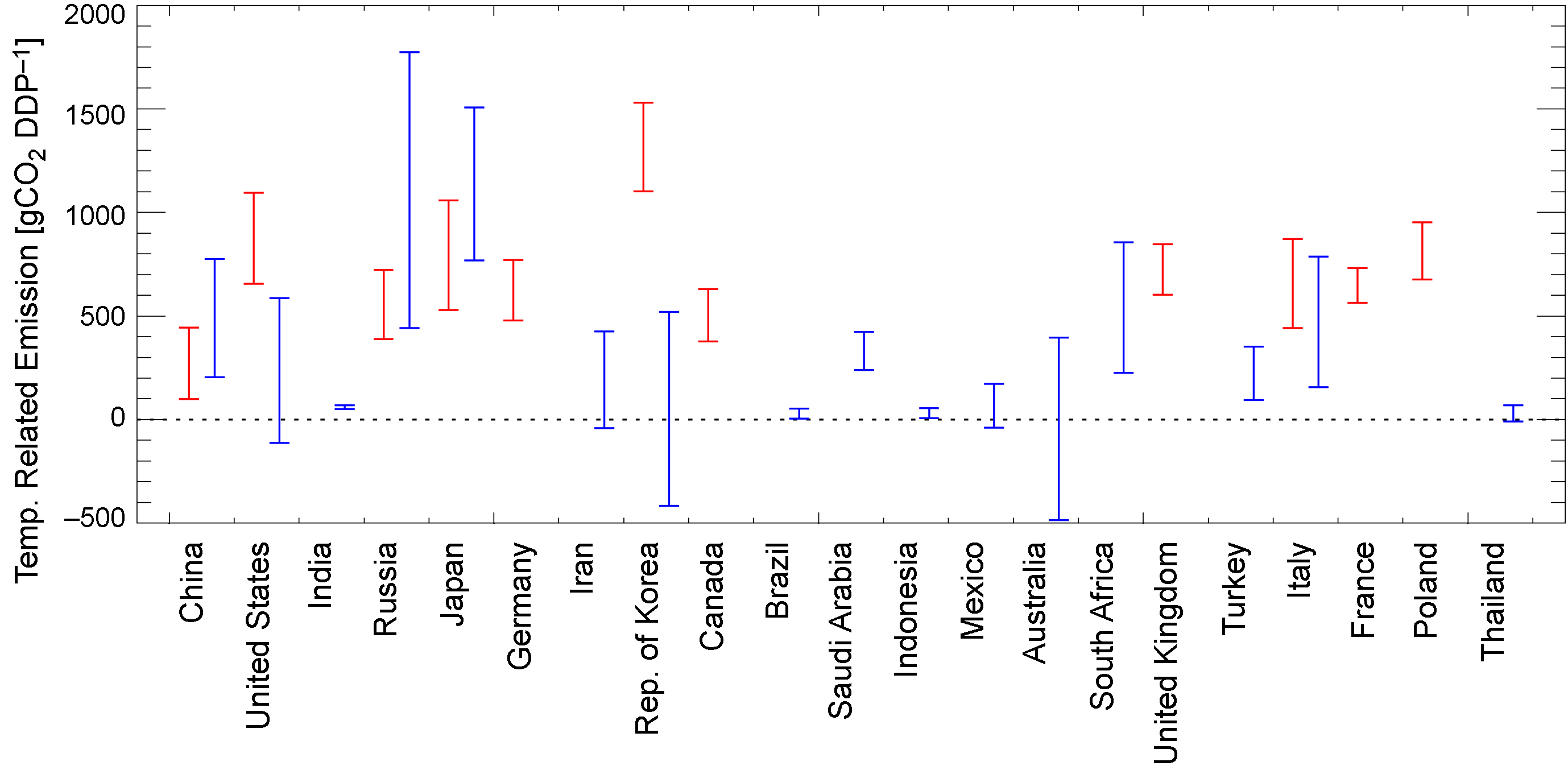
Figure 3 Estimates of the heating and cooling-related CO2 emissions for the 20 most emitting countries. The figure shows the results of the linear fit analysis as shown in figure 2. The temperature-related emissions are given in g CO2 per degree-day-person (i.e. heating-degree-day-person in red and cooling-degree-day-person in blue).
Download figure:
Standard image High-resolution imageFigure 3 shows that the CO2 emissions associated with heating are on the order of 500–1000 gCO2 per degree-day-person for mid-latitude countries. Canada, a country notable for harsh winters, shows lower values, which might be related to a better home insulation adapted to the local climate. China also shows a sensitivity that is lower than that of other mid-latitude countries, while the opposite is true for South Korea. The CO2 emissions associated with cooling show a larger diversity. Interestingly, several subtropical countries (India, Indonesia, Brazil, Thailand) show very small sensitivities to CDP (a few tens gCO2 CDP−1) with small uncertainties, possibly indicating a small penetration of air conditioning. The two largest emitters, China and the United States, have retrieved estimates for both heating and cooling, but the cooling uncertainty range is large and encompasses the null value for the latter. This low sensitivity to CDP is surprising and contradicts earlier results. For instance, Hao et al (2016) concludes that CO2 emissions in China are more sensitive to CDD than to HDD. For the United States, Hadley et al (2006) indicates that cooling is less energy efficient than heating, so an increase in cooling needs (and associated fossil-fuel carbon emissions) can more than offset an equal decrease in heating needs (and associated fossil-fuel carbon emissions). Our results for the cooling sensitivity are therefore suspicious.
As a sensitivity analysis, we have perturbed the time series of HDP and CDP, and applied the same regression tools. One test uses the fully randomized time series of HDP/CDP, while another swapped the values of each odd and its following even years. The latter method retains the long-term trend in the time series but de-correlates the year-to-year variations. In both cases, the correlations are much less than those shown above and no consistent CO2 emission sensitivity to the temperature is found. This simple analysis provides strong evidence that the correlations and retrieved sensitivity are not spurious.
Figure 4 is an analysis of the annual growth rate of CO2 emissions for the same countries as in figure 1 and figure 2. It shows the various components that contribute to the growth rate (in a given year relative to the previous year), according to our simple model. The components are the GDP, the energy intensity, heating and cooling. Note that the ranges vary markedly between countries so that we use different scales that are indicated on the right side within each subplot. This figure shows that the inter-annual variations of the meteorology have a small but discernible influence on the CO2 emission growth rate. This influence appears particularly significant for Germany, South Korea and Japan (figure 4), as well as the United Kingdom, Italy, France and Poland (supplementary figure S-3). The model however is far from perfect as the actual growth rate (diamond symbols) sometimes differs significantly from the sum of the components (horizontal white bar). Some uncertainty on the input data may also contribute to the discrepancies. For the seven countries cited above, for which the relative contribution of heating/cooling is the largest, there is a rather good agreement between the modelled CO2 growth rate and its true value. One conclusion that can be derived from this figure is that the strong decrease of Germany's emissions in 2014 was for a large part due to a mild winter, confirming previous findings (EEA 2015). Indeed, the winter of 2014 was near record warmth in Europe and its impact on the emissions can be seen on the figure 4 subplot for Germany, but also for the United Kingdom, France, Italy and Poland (figure S-3).
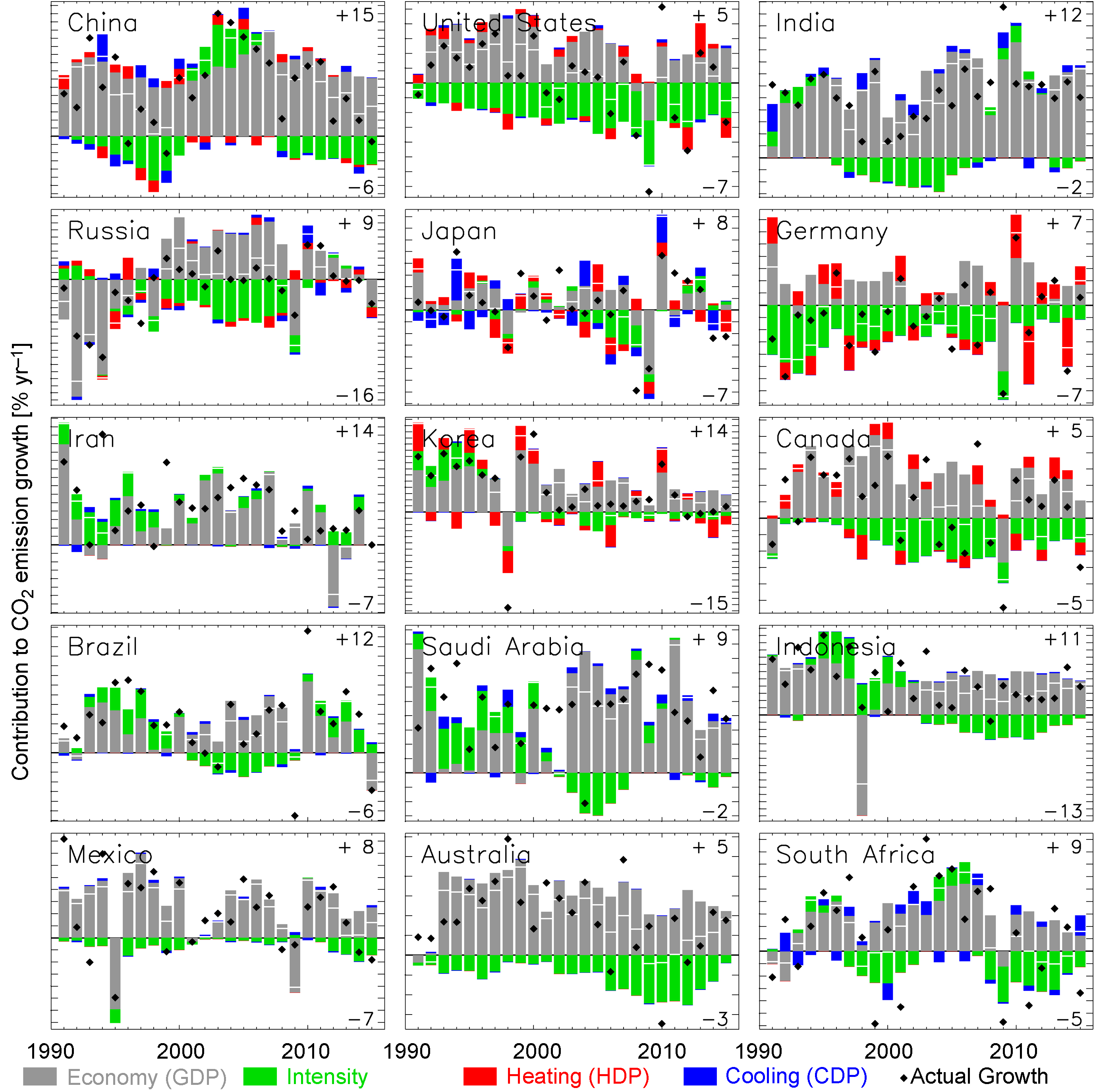
Figure 4 Decomposition of the annual (year-on-year) growth rate of the CO2 emission related to the variation of the economy (quantified by the GDP), the economy intensity and the fraction related to heating and cooling. The actual growth rate of EMICO2 is shown by a diamond symbol whereas the model estimate (i.e. the sum of the four terms) is indicated by a white horizontal bar. Note that the scales are different for each figure. The tick marks are for 1% growth rate and the scale is indicated on the right side of each figure. A similar figure for the next 15 countries is shown in the supplementary material.
Download figure:
Standard image High-resolution imageThe results derived at the country level can be aggregated to analyse the impact of inter-annual meteorology on the CO2 emissions at the global scale. For this objective, we use the heating and cooling sensitivity convolved by the HDP and CDP time series. The uncertainties are also aggregated assuming that the errors for the various countries are independent. When the estimate was unsuccessful, we assume that there is no CO2 emission related to heating or cooling. There are also some countries for which the GDP data is incomplete so that our analysis could not be applied to them, but these countries contribute a very small fraction of the total emissions. The results of the aggregation are shown in figure 5. According to our analysis, heating related emissions contribute slightly above 3 ± 0.5 GtCO2 per year, which is about 10% of the total fossil fuel emissions. Overall, the share of cooling and heating emissions are broadly consistent with their share in final energy consumption in 2010 according to Labriet et al (2015) (10.4%) and the share estimated by Isaac and van Vuuren (2009) with a much more detailed model (nearly 3 GtCO2 for domestic heating and cooling only). There are inter-annual variations of a few tenths of GtCO2. Cooling related emissions, around 0.45 ± 0.35 GtCO2 per year, are much smaller than those of heating but show a significant positive trend. Note however that the general trend for the cooling emissions is 0.4 GtCO2 from 1990 to 2014, which is the order of magnitude of the interannual variations of the heating emissions. Both population increase and global warming contribute to the positive trend on the cooling emissions. Conversely, the impact of global warming on the heating-related emissions and that of the population growth are opposite in sign and tend therefore to compensate. This explains that the relative trend on the cooling-related emissions is much larger than that of the heating-related emissions (figure 5). Penetration of air conditioning plays a role as well, but cannot be captured by our simple modelling approach. However, even in more detailed modelling attempts, such as the one conducted by Isaac and van Vuuren (2009) for the building sector, this is not expected to play a major role on heating and cooling induced fossil-CO2 emissions over the period covered by our analysis (see their figure 7).

Figure 5 Heating (left) and cooling (right) related CO2 emission anomalies according to our analysis for the world total. The uncertainties are estimated assuming that each country uncertainty is independent (quadratic sum).
Download figure:
Standard image High-resolution imageFigure 6 is similar to the subplots in figure 4 but for the total of the 108 countries considered in our analysis. This total differs from the world total given in EDGAR because it does not include emissions from the few countries excluded from our analysis for lack of GDP data, and the so-called 'bunkers'. This comes in addition to the slight differences with the national time series provided by CDIAC. As a result, our growth rates differ slightly from those of CDIAC. In particular our growth rates for the countries considered are 2.2, 1.1 and −0.1% for 2012/2013, 2013/2014 and 2014/2015, respectively, whereas they are 1.3, 0.8 and 0.1% for the CDIAC 'World' emissions discussed in Le Quéré et al (2015, 2016). Figure 6 shows that the increase in emissions is mostly fuelled by the economic growth quantified by the GDP, partly compensated by a decrease in the emission intensity of the economy. The inter-annual variations of the GDP are large and represent the main driver of variations in CO2 year-on-year emission growth rate. Heating and, to a lesser extent, cooling also contribute to the inter-annual variation of the growth rate. There was a significant decrease of the emission growth rate in 2014, which was attributed to the slowdown of the Chinese economy and a gradual shift from coal to renewable energy (Green and Stern 2015, Jackson et al 2015). This slowdown was recently confirmed with the release of 2015 emissions (Le Quéré et al 2016). The heating-related emissions of 2014 are significantly smaller than those of 2013 by 150 ± 50 MtCO2, while the cooling emissions are also smaller by ≈70 MtCO2. The sum of these decreases represents about 0.5% of total emissions. In 2015, heating related emissions decrease by an additional 80 MtCO2, partly compensated by an increase of the cooling emissions (figure 5). Our analysis thus indicates that meteorology was a significant factor, explaining about half of the 2013 to 2014 emission growth reduction. Note that the true emission growth (diamond symbol) for the three most recent years is well reproduced by our simple model (white horizontal bar) while it is not the case for a few earlier years. The discrepancies for these years confirm that other factors for the CO2 growth rate have had a significant influence that is unaccounted for in our simple analysis. Nevertheless, our analysis indicates a significant contribution of meteorological effects to the decrease of the CO2 emission growth rate from 2013 to 2014, and a small but no significant impact from 2014 to 2015.

Figure 6 Decomposition of the annual (year-on-year) growth rate of the CO2 emission related to the variation of the economy (quantified by the GDP), the economy intensity, and the fraction related to heating and cooling. The actual growth rate of EMICO2 is shown by a diamond symbol whereas the model estimate (i.e. the sum of the four terms) is indicated by a white horizontal bar.
Download figure:
Standard image High-resolution image
4. Conclusions
Our analysis confirms that time series of national CO2 emissions from 1990 to 2015 exhibit a close relationship with gross domestic product (GDP) modulated by the slow-changing carbon intensity of the economy. The inter-annual variations in CO2 emissions that are not explained by the change in GDP, are positively correlated to HDP and/or CDP for many countries, with slopes of typically 500–1000 gCO2 (degree-day-person)−1 but with significant country-to-country variations. The inter-annual anomalies of the meteorology contribute significantly to year-on-year variations in the CO2 emission growth rates, in particular for mid-latitude countries.
We acknowledge several shortcomings and uncertainties in our modeling and results. First, the input time series convey some uncertainties and we have not attempted to quantify their impact on the results. Second, there may be hidden correlations between the time series that are not properly accounted for in the modeling. For instance, the meteorology anomaly may impact the GDP and emissions in ways that are not related to heating and cooling. An example is the precipitation anomalies that drive the hydro-electricity potential, and therefore the need to use coal power plants as a substitute. Another example is the fact that (bad or good) weather is known to affect consumption and GDP. Finally, we have hypothesized that the heating and cooling emissions are proportional to the HDP and CDP with arbitrary definition of temperature thresholds. In practice the typical usage of heating and cooling devices may change with time: on the one hand, the surface heated or cooled per inhabitant may increase; on the other hand the average home insulation may improve; finally the fossil carbon content of the energy may change over time together with the use of fossil fuels in replacement of traditional biomass or the development of renewables and/or electrification combined with low-carbon sources of electricity. Clearly, there are more accurate ways to quantify the carbon content of heating and cooling, but these would require the use of detailed statistics at the country scale.
Despite these admitted limitations, we have used the HDP and CDP-dependent emission sensitivity inferred from the national time series to aggregate the emission anomalies at the global scale. The heating- and cooling-related emissions of 2014 are significantly smaller than those of 2013 by 220 ± 60 MtCO2, which represents about 0.5% of the total emissions. Thus, about half of the change in emission from 2013 to 2014 can be explained by temperature factors. Changes in heating- and cooling-related emissions are marginally smaller in 2015 as compared to 2014 and represent a rather small contribution to the limited growth in 2015.