
Abstract
The temperature response of atmosphere–ocean climate models is analyzed based on atmospheric CO2 step-function-change simulations submitted to phase 5 of the Coupled Model Intercomparison Project (CMIP5). From these simulations and a control simulation, we estimate adjusted radiative forcing, the climate feedback parameter, and effective climate system thermal inertia, and we show that these results can be used to predict the temperature response to time-varying CO2 concentrations. We evaluate several kinds of simple mathematical models for the CMIP5 simulation results, including single- and multiple-exponential models and a one-dimensional ocean-diffusion model. All of these functional forms, except the single-exponential model, can produce curves that fit most CMIP5 results quite well for both continuous and step-function CO2-change pathways. Choice of model for any particular application would include consideration of factors such as the number of free parameters to be constrained and the conception of the underlying mechanistic model. Smooth curve fits to the CMIP5 simulation results realize approximately half (range 38%–61%) of equilibrium warming within the first decade after a CO2 concentration increase, but approximately one quarter (range 14%–40%) of equilibrium warming occurs more than a century after the CO2 increase. Following an instantaneous quadrupling of atmospheric CO2, fits to four of the 20 simulation results reach 4 ° C of warming within the first decade, but fits to three of the 20 simulation results require more than a century to reach 4 ° C. These results indicate the need to reduce uncertainty in the temporal response of climate models and to consider this uncertainty when evaluating the risks posed by climate change.
Export citation and abstract BibTeX RIS

Content from this work may be used under the terms of the Creative Commons Attribution 3.0 licence. Any further distribution of this work must maintain attribution to the author(s) and the title of the work, journal citation and DOI.
1. Introduction
Recent studies of state-of-the-art atmosphere–ocean general circulation models (AOGCMs) have found that, when presented with an abrupt increase in atmospheric carbon dioxide concentration, the various models project a relatively wide range of values for the equilibrium temperature change (ΔTeq) that is expected to be approached after more than a century. Andrews et al [1], for example, reported that estimated values for the equilibrium climate sensitivity (i.e., the increase in global mean air temperature near the surface, once equilibrium has been restored following an abrupt doubling of atmospheric CO2 concentration) range from 2.08 to 4.67 ° C, with the spread attributable in large part to cloud radiative effects.
This divergence in long-term projections among advanced AOGCMs suggests that the models may also differ substantially in their projections of the pace of warming following a rapid increase in CO2 levels, a subject of obvious relevance to climate policy. Some studies (e.g., [2, 3]) have analyzed transient climate response as a process that involves two distinct time scales: a fast response that corresponds to the rapid warming of the land and upper ocean, and a slower component that represents the warming of the deeper ocean. Other studies [4, 5] have put forth simpler climate models, such as one-dimensional ocean models that use a heat-diffusion equation with a linear-radiative upper boundary condition to estimate the dynamics of warming; these models do not involve multiple time scales that are clearly separated from one another, in contrast to conclusions drawn by Held et al [2].
Here we examine the time evolution of global warming as projected by all 20 AOGCMs participating in phase 5 of the Coupled Model Intercomparison Project (CMIP5) that have contributed results consistent with the abrupt4xCO2 protocol by 16 March 2013 [6, 7]. Our study focused on simulation results for the abrupt4xCO2 protocol, which instantaneously quadruples the concentration of atmospheric CO2 from a near-equilibrium, preindustrial state of about 285 ppm to about 1140 ppm. Although such a dramatic change is not realistic, simulating a step-function increase of this kind can reveal fundamental climate system properties that are often difficult to disentangle in more complicated scenarios. The abrupt4xCO2 simulations were analyzed by Andrews et al [1], for example, to estimate the climate feedback parameter in these models by applying the methodology of Gregory et al [8]. Previous studies [9, 10] give some basis for confidence that the simulated climate behavior illuminated by the abrupt4xCO2 simulations are also applicable to more realistic scenarios.
In this work, we characterize the transient response observed in these simulations in several ways. Using the most complete data sets available, we replicate and extend the analysis of Andrews et al to estimate, for each of the 20 models, the ultimate equilibrium warming resulting from the quadrupling of CO2. We then fit multi-exponential curves and a highly schematic one-dimensional heat-diffusion ocean model to the model results. These fits allow us to compare the warming values projected by the suite of models at various intermediate time points and to test whether or not separate time scales are required to approximate climate responses to sudden changes in forcing. Lastly, we apply some of the same analytical methods to CMIP5 simulations run on the 1pctCO2 protocol, in which atmospheric CO2 increases by 1% each year, and we examine whether the simpler one-dimensional diffusion climate model gives reasonable projections of the pace of warming for this more realistic scenario.
2. Methods
2.1. Climate model data
Monthly mean data available on 16 March 2013 were obtained for all models in the CMIP5 ensemble output for three separate experiments: piControl, a fully coupled control model of the preindustrial climate; abrupt4xCO2, which instantaneously quadruples atmospheric CO2 content from the preindustrial value; and 1pctCO2, which increases the atmospheric CO2 concentration by 1% yr−1, starting from the preindustrial control value. We made use of the entire duration of simulation data supplied, which ranges in length from 140 to 300 years; our results thus extend those of previous studies that were performed when only a subset of this data was available [1]. For data from the abrupt4xCO2 and 1pctCO2 experiments, we first calculated annual mean values and then calculated differences from the preindustrial values by subtracting a LOESS fit [11] (from a locally weighted polynomial regression with 100 year width) to the piControl simulation. Little difference was found in the results when linear fits to the control simulations were subtracted instead, as was done in [1]. In this letter, references to results of the abrupt4xCO2 and 1pctCO2 simulations refer to results with the control simulation subtracted in this way.
2.2. Linear fits to estimate radiative parameters
Our principal analysis used data from the abrupt4xCO2 simulations to diagnose the parameters most central to the dynamic response of the 20 AOGCMs: the adjusted radiative forcing (F), the climate feedback parameter (λ), and the equilibrium temperature change (ΔT4×). 'Adjusted radiative forcing' refers to the top-of-atmosphere radiation imbalance that exists after the atmosphere and land surface have adjusted to changes in greenhouse gas concentrations but before there has been an appreciable change in global mean temperature [1, 8, 12].
Following Andrews et al [1], we used the method of Gregory et al [8] and performed a linear regression on global net downward top-of-atmosphere radiative flux (R) against change in global mean temperature (ΔT) at the reference height of 2 m above all surfaces. We make the linear approximation

After centuries or millennia of warming in response to the four-fold increase in CO2, the top of the atmosphere approaches net radiative equilibrium (i.e., R = 0), and the total amount of temperature change approaches its equilibrium value:

It should be noted that there is some evidence of curvature exhibited in the CMIP5 data (SOM figure S1, available at stacks.iop.org/ERL/8/034039/mmedia) used in the regressions for equation (1). However, to minimize the number of free parameters and arbitrary assumptions, we apply a linear analysis here. We assume that this could introduce errors in estimated parameter values on the order of about 10%.
2.3. Curve fits to estimate temporal parameters
To analyze and compare the detailed trajectories of the global warming that the CMIP5 models project would follow a rapid increase in CO2 levels, we fit four different curves to the annual mean temperature increases derived from the abrupt4xCO2 simulation data sets. First, we divided the temperature increase (ΔT) in year t by the equilibrium temperature change to obtain a dimensionless temperature-response function:
We then fit curves of the form


and

As t increases, the temperature increase ΔT approaches the asymptote ΔT4×. This implies

Thus, we impose a constraint on equation (5) that θ0 + θ1 = 1, and on equation (6) that θ0 + θ1 + θ2 = 1. Note that this functional form and this constraint also imply that at time t = 0,θn-exp(t) = 0. We find values of the coefficients θi, as well as of the exponential parameters τi, in equations (4)–(6) that minimize the time-integrated variance between θ(t) and each of these functions; the resulting values are listed in SOM tables S3–S5 (available at stacks.iop.org/ERL/8/034039/mmedia). Equations (4)–(6) can be interpreted as representing solutions to one-, two-, and three-box models of heat uptake (see, for example, [13] for a physical interpretation of a 2-exp fit), but we fit values as a purely formal exercise. (A physics-based fit could constrain asymptotic heat uptake with the known heat capacity of the ocean.)
We also consider a fourth kind of curve that is based on the simple one-dimensional heat-diffusion climate model of Hansen et al [14]. Such models represent the ocean as a vertical diffusive column [15] and assume that outgoing long-wave radiation varies linearly with surface temperature [16]. In such a model (see examples in [4, 14, 17]), the top-of-atmosphere net radiative fluxes, which follow equation (1), are applied to a one-dimensional slab representing the heat capacity of the climate system (primarily the oceans), subject to a zero-flux boundary condition at the maximum depth (zmax), which we take to be 4000 m:


where θκ(z,t) represents the normalized temperature as a function of depth, ρ = 1025 kg m−3 is the density of sea water, and cp = 3993 J kg−1 K−1 is the heat capacity of sea water. For notational convenience, we specify θκ(t) = θκ(0,t) and θκ(t) = ΔT(t)/ΔT4×. With these specifications, only the vertical thermal diffusivity parameter κv remains to be determined from the fits to θ(t), which were calculated by least-square regression against the CMIP5 simulation results as described above.
We refer to the curve fits obtained by using equations (4)–(6) as 1-exp, 2-exp, and 3-exp fits, respectively, and to the curve fit using the solution of equations (8)–(10) as the 1D fit. When reporting results for models at specific times, we use 3-exp fits from equation (6) to filter high-frequency variability in the AOGCM model results.
2.4. Simulations of a steady increase in CO2 levels
We performed simulations to test the extent to which the curve fits discussed above can approximate the AOGCM results for the 1pctCO2 simulations. The temporal dynamics exhibited for step-function changes in radiative forcing are also at play in simulations of transient climate change, and step-function simulations can therefore be used to parameterize a simple climate model to make good predictions for the more complex climate model's response to transient changes in radiative forcing [9]. Indeed, transient climate change may be numerically approximated as the superposition of a large number of small, step-function changes in radiative forcing, such as by the CMIP5 1pctCO2 protocol, which assumes that atmospheric CO2 content increases at a rate of 1% yr−1 from the preindustrial value of 285 ppm.
In these simulations, radiative forcing varies over time. We assumed that the adjusted radiative forcing is proportional to the radiative forcing for CO2 based on the formula used by the IPCC [18] (see SOM section S1, available at stacks.iop.org/ERL/8/034039/mmedia). This formulation is more complicated than, but yields results that are similar to, the more commonly applied log-like dependence of CO2-radiative forcing on atmospheric CO2 concentration. If we use FIPCC to denote the radiative forcing for CO2, and F4× represents the adjusted radiative forcing determined above from the abrupt4xCO2 simulations (table S1, available at stacks.iop.org/ERL/8/034039/mmedia), then we can represent the adjusted radiative forcing F(c) as a function of CO2 concentration c as

where FIPCC(c4×) = 8.52 W m−2.
In our simulations, we used the values determined above for the parameters F,λ, and κv. In our simulations that used the multi-exponential approach to predict temperature changes, we applied a convolution integral approach, wherein the temperature change ΔT at time t is estimated as

where θn-exp(τ) in equation (12) represents either the 1-exp, 2-exp, or 3-exp curve fits to temperature changes in the abrupt4xCO2 simulations, as described above. For the 1D model represented by equations (8)–(10), we performed a numerical simulation. Over time scales ranging from a few years to a century, this model behaves similarly to the analytic solution to a one-dimensional, semi-infinite diffusive slab experiencing a step-function increase in radiative forcing [5].
3. Results and discussion
3.1. Radiative parameters and equilibrium temperature change
Values of λ,F4×, and ΔT4× calculated from the linear regression to the output from the 20 CMIP5 models that had submitted results from abrupt4xCO2 simulations are illustrated in figure 1. Numeric values and uncertainty estimates are presented in SOM table S1 (available at stacks.iop.org/ERL/8/034039/mmedia), and data with curve fits are plotted in SOM figure S1 (available at stacks.iop.org/ERL/8/034039/mmedia). The values we obtained are very similar to those reported by Andrews et al [1], and the minor differences mainly reflect the consideration in our study of all simulated years submitted by the modeling groups. Values for radiative forcing (F4×) ranged from 5.2 to 8.6 W m−2 and had a median value of 6.6 W m−2. Values for the climate sensitivity parameter ranged from 0.63 to 1.55 W m−2 K−1 (SOM table S1). Values for estimated equilibrium warming (F4×) ranged in these simulations from 4.1 to 9.3 K, similar to values obtained by Andrews et al [1].
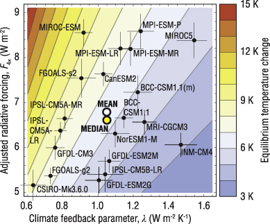
Figure 1. The climate feedback parameter (λ, horizontal axis), adjusted radiative forcing (F4×, vertical axis), and equilibrium temperature change (ΔT4×, contours) for the 20 models submitting output to CMIP5, as calculated from abrupt4xCO2 simulations that posit an instantaneous four-fold increase in atmospheric CO2 concentration. Median and mean values represent the median and mean values of λ and F4× determined by fits to each individual model. Crossed lines indicate 95% confidence intervals. Numeric values are presented in SOM table S1 (available at stacks.iop.org/ERL/8/034039/mmedia).
Download figure:
Standard image High-resolution imageFigure 1 illustrates the wide dispersion among the models of these values around the mean and median. It should be noted that the model having the median value may differ depending on field, parameter, or time considered; there is thus no one 'median model' defined here. Radiative forcing, and thus warming, following a doubling of atmospheric CO2 would likely be approximately half as large as that shown here [18].
3.2. Pace of warming in abrupt4xCO2 results
The projected warming at t = 100 years after the step-function quadrupling of CO2 concentration varied from 3.0 to 6.5 ° C; the median warming at 100 years was 5.0 ° C (SOM table 2, available at stacks.iop.org/ERL/8/034039/mmedia). To enable more meaningful comparison among the models of the temporal dynamics of the warming, we rescaled the trajectories in figure 2 so that the left vertical axis represents the fraction of the ultimate equilibrium temperature change projected by each model (i.e., ΔT/ΔT4×). The top of each panel in figure 2 is thus the asymptote for the multi-exponential curve.
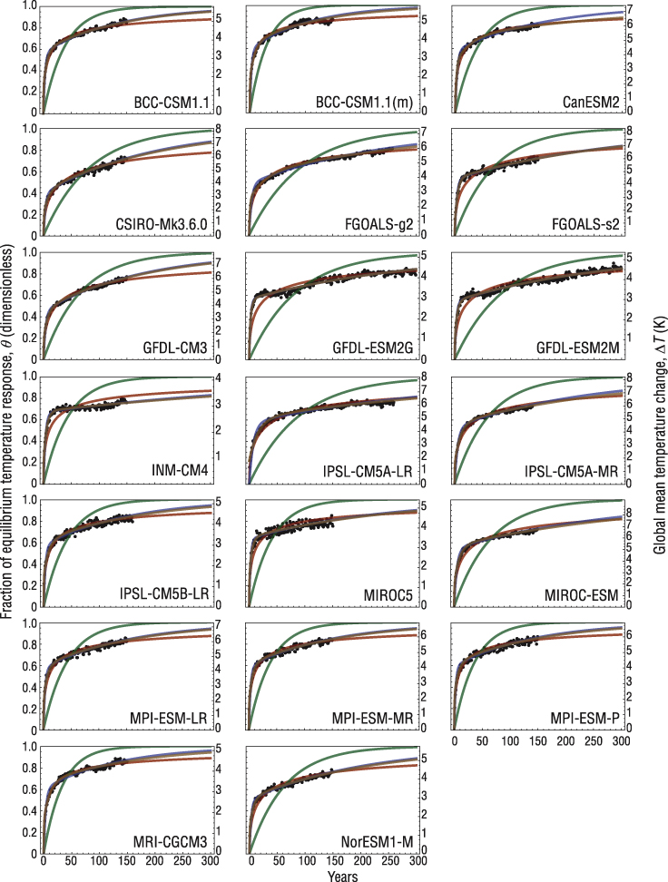
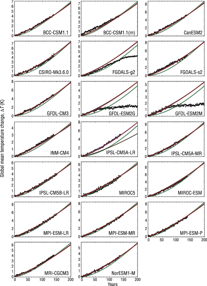
Figure 2. Temperature results for CMIP5 models that have performed the abrupt4xCO2 simulations (black dots). Also shown are fits to this data using the functions described in the text: θ1-exp, green; θ2-exp, blue; θ3-exp, brown; θ1D, red. The left vertical axis shows the fraction of equilibrium temperature change (i.e., ΔT/ΔT4×); the right vertical axis indicates the absolute change in global mean temperature. Fit parameters are listed in SOM tables S3–S5 (available at stacks.iop.org/ERL/8/034039/mmedia).
Download figure:
Standard image High-resolution imageIt is evident from figure 2 that some models in this ensemble project much more rapid warming than others do. At the 10 year mark, the median model had realized 54% (range 38%–61%) of its ultimate equilibrium temperature change; by year 100 of the simulations, the median model had realized 71% (range 60%–86%) of the equilibrium temperature change (figure 3 and SOM table S2). At the 10 year mark, the median model had warmed 3.2 ° C (range 2.4–4.3 ° C); by year 100 of the simulations, the median model projected 5.0 ° C (range 3.0–6.1 ° C) of warming. The inference from the abrupt4xCO2 results is thus that about half the equilibrium climate change occurs in the first decade after a change in forcing but about a quarter of global warming would occur more than a century into the future. The range of model predictions tend to diverge in time, both in an absolute sense—maximum projected values exceeded minimum values by 1.9 ° C after 10 years, 3.1 ° C after 100 years, and 5.2 ° C in equilibrium—and in relative terms: maximum projected values exceeded minimum projected values by 61% after 10 years, 141% after 100 years, and 182% in equilibrium. Results for the climate feedback parameter, effective vertical thermal diffusivity, and fraction of climate change attained 10 and 100 years into the simulations are plotted in figure 4.
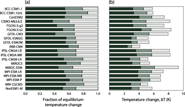
Figure 3. (a) Fraction, and (b) amount, of equilibrium climate change realized between 0 and 10 years after a step-function-change in CO2 concentration (dark green), between 10 and 100 years after the change (medium green), and more than 100 years after the change (light green) for the climate models that have performed the CMIP5 abrupt4xCO2 simulation.
Download figure:
Standard image High-resolution image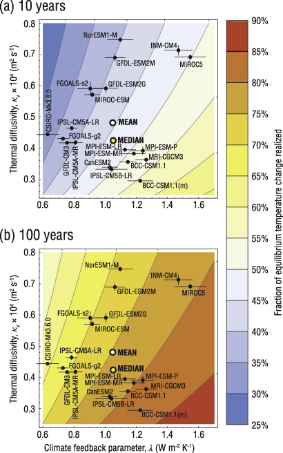
Figure 4. Results for climate feedback parameter (λ, horizontal axis), effective vertical thermal diffusivity (κv, vertical axis), and fraction of climate change (contours) realized (a) 10 years and (b) 100 years after a step-function quadrupling of atmospheric CO2 content; results shown here were derived by using the one-dimensional model described in the text, which can differ from the other curve fits by about 5%. Crossed lines indicate 95% confidence intervals. Numeric values are listed in SOM tables S1 and S2 (available at stacks.iop.org/ERL/8/034039/mmedia).
Download figure:
Standard image High-resolution image3.3. Comparison of different curve fits to abrupt4xCO2 and 1pctCO2 results
Results of curve fits to the annual mean warming in the CMIP5 abrupt4xCO2 results are plotted in figure 2; curve fits to the 1pctCO2 results are plotted in figure 5. Figure 2 shows a strong degree of concordance among the 2-exp, 3-exp, and 1D fits, especially at times after year 50 of the simulations. In contrast, the exponential fit with a single time constant (1-exp) failed to capture rates of change on both decadal and century scales [2].
Figure 5. Results from CMIP5 models (black dots) running simulations of the 1pctCO2 protocol. Projections made by simulations based on curve fits to the abrupt4xCO2 simulations as described in the text: θ1-exp, green; θ2-exp, blue; θ3-exp, brown; θ1D, red. All but θ1-exp provide similar approximations to the temperature results for most of the fully coupled, three-dimensional climate model simulations. Note that the GFDL-ESM2G and GFDL-ESM2M models did not continue with increasing atmospheric CO2 content after reaching twice the preindustrial concentration.
Download figure:
Standard image High-resolution image
Held et al [2] suggested a conceptual model for temperature change wherein the approach to equilibrium may be considered as the sum of two terms: a rapidly adjusting term that equilibrates exponentially on a time scale of less than 5 years, and a second component that adjusts on a much longer time scale. Jarvis [3] analyzed the response of three climate models to a rapid exogenous forcing and suggested that their equilibration may be affected by positive feedbacks having time scales ranging from a decade to a millennium. Our results, however, suggest that the goodness of fit of a function involving two-exponential time constants does not, in itself, provide strong evidence for two underlying physical processes having two distinct time scales. We suggest that these curve fits be considered pragmatically and assessed based on their utility for specific applications. For some purposes, consideration of a single process (as in the 1D model) may be sufficient—and where a closer correspondence to the fitted data would be useful, it may be necessary to consider more than two time scales (as in the 3-exp fit).
To evaluate and rank the quality of the 1-exp, 2-exp, 3-exp, and 1D fits to the abrupt4xCO2 CMIP5 model results, we employed the corrected Akaike information criterion (AICc) [19]. AICc is an information-theoretic measure that takes into consideration the goodness of fit and number of free parameters, and ΔAICc is often used as an objective criterion for model selection [19]. By this selection criterion, we found that the 3-exp curve provided the best fits to the abrupt4xCO2 simulations for all 20 CMIP5 models considered here (table S6, available at stacks.iop.org/ERL/8/034039/mmedia). We note that with the constraints outlined above, the 1-exp, 2-exp, 3-exp, and 1D fits have one, three, five, and one free parameters, respectively. We speculate that the 3-exp fits were better able to represent the rapid adjustment of land-surface (and land-plant) temperatures. Indeed, substantial temperature changes over land are observed to occur within days in climate model simulations of step-function changes in radiative forcing [20]. The median value of the shortest time constant in the 3-exp fits was 0.6 years, which is less than the annual resolution used in this analysis. Our examination of the second-best fits, as evaluated by ΔAICc, found that the 2-exp fit was better than the 1D fit in the cases of 13 of the 20 models considered. For simulation results from all 20 models, the 1-exp fit yielded the worst fits among the curve equations considered. Apart from the 1-exp fits, all of the functional forms considered here yield fair approximations of the global and annual means resulting from the three-dimensional model runs. Our point is not that the ΔAICc clearly demonstrates that one functional form is better than another, but rather that curve-fitting alone does not clearly select for one functional form over another. The choice of functional form for the curve fit therefore cannot be seen as strong evidence for the 'correctness' of a specific underlying conceptual model of the physical processes.
We also used ΔAICc to rank the ability of the 1-exp, 2-exp, 3-exp, and 1D fits to predict the results of the 1pctCO2 simulations based on the fits of these equations to the abrupt4xCO2 results (table S7, available at stacks.iop.org/ERL/8/034039/mmedia). We found that, by this criterion, the best predictions of the 1pctCO2 results were produced by the 1D fits for 8 of 17 models, by the 2-exp fits for 6 of 17 models, and by the 3-exp fits in 3 of 17 models. (As of our accession date, 17 CMIP5 models had simulation results available in which atmospheric CO2 concentrations increased by 1% throughout the entire simulation.) Our comparison of 2-exp to 1D fits found that the 2-exp fits ranked higher for 8 of 17 models; the 1D fits ranked higher for the remaining 9 models.
We also ranked models by calculating the root-mean-square residual error (RMSE) of the predictions, without considering the number of degrees of freedom in the fit (table S8, available at stacks.iop.org/ERL/8/034039/mmedia). Predictions for 1pctCO2 based on the 1-exp fits to the abrupt4xCO2 results had a median RMSE of 0.31 ° C (range 0.21–0.87 ° C). The 2-exp fits had a median RMSE of 0.13 ° C (range 0.10–0.34 ° C). The 3-exp fits had a median RMSE of 0.16 ° C (range 0.10–0.34 ° C except for one outlier at 1.00 ° C). The 1D median RMSE was 0.15 ° C (range 0.09–0.32 ° C).
Under these two tests of predictive utility—ΔAICc and RMSE—the 1D fit performed similarly to the 2-exp fit, despite having one degree of freedom rather than three. The 2-exp and 3-exp fits could, in principle, be constrained by specifying the implied heat capacity of the climate system; this constraint would reduce by one the number of degrees of freedom of each of these models. For many purposes, it may be a sufficient approximation to use a one-dimensional heat-diffusion ocean model having just one degree of freedom—in effect, to approximate warming as a simple heat-diffusion process. However, the 2-exp and 3-exp curve fits did provide a better fit to some of the model data sets, most notably in the first 50 years.
The time scale required for temperature equilibration is affected by the value of λ, but the different functional forms imply different relationships between this time scale and λ. The time constant in the 1-exp fit, for example, is proportional to λ−1, whereas a semi-infinite version of the one-dimensional diffusive model has a time constant that is proportional to λ−2 [17]. Held et al [2] found that the faster of the two time constants in the 2-exp fit is proportional to (λ+k0)−1 and the slower time constant is proportional to k1 + λ−1, where k0 and k1 are positive constants. To the extent that CMIP5 abrupt4xCO2 and 1pctCO2 simulations can be well approximated by linear models [9], we would expect the time constants associated with warming to be independent of the size of the forcing, whereas the amount of warming should scale approximately linearly with the forcing. We note, however, that our conclusions for the 1pctCO2 results may not be relevant to all possible scenarios; results may differ if forcings are stable or reduced.
3.4. Rapid adjustment
A step-function change in radiative forcing initiates a chain of events that occur on a broad spectrum of time scales (e.g., atmospheric adjustment, adjustment of land plants, land-surface temperature adjustment, near-surface ocean adjustment, ocean thermocline adjustment, deep ocean adjustment) [20]. The 3-exp fits to annual mean data (SOM table S5, available at stacks.iop.org/ERL/8/034039/mmedia), involve three time distinct scales. The most rapid time constants obtained have a median value of 0.68 years (range 0.25–2.9 years). A median of 23% (range 8%–46%) of equilibrium temperature change is approached on this most rapid time scale. Rapid heating of land may contribute to the shortness of the regression time constant.
4. Conclusions
4.1. Implications for simple models
Atmosphere–ocean GCMs require large amounts of computation and involve a larger set of assumptions than can be held in any one human mind. They are thus impractical to use for many kinds of study where rapidity of computation or explicit exposition of assumptions is of paramount importance. The methodology of Gregory et al [8] and related approaches can be used to define constants for simple climate models. These simple models approximate certain behaviors of the AOGCM, and can be useful tools in economic or other analyses.
'[A]ll models are wrong, but some are useful' [21]. The evaluation of simple climate models is a search for simple climate models that are likely to be useful in contexts where running sets of full GCM simulations is impractical. We have compared four different candidate models, which we trained on results of the CMIP5 abrupt4xCO2 experiment and then tested against results of the 1pctCO2 experiment (SOM tables S6–S8, available at stacks.iop.org/ERL/8/034039/mmedia). We conclude that there are few, if any, circumstances in which a single-exponential model, which has only one free parameter, is likely to appropriately balance accuracy of representation and conceptual simplicity. We find that when just one free parameter is desired, the response of the climate to a change in radiative forcing can be much more closely approximated by a heat-diffusion climate model [4, 5, 14, 15] in which the free parameter represents the constant vertical thermal diffusivity of heat-diffusion in the ocean. This result suggests that consideration of just one underlying process could predict most of the trend in global and annual temperature. For many of the models participating in CMIP5, an improved fit to the abrupt4xCO2 experiment results can be obtained with a two-exponential fit, which can be treated conceptually as a two-box ocean model [1, 2]. This two-exponential model, which has three free parameters, produces better fits than the 1D model for a majority of the CMIP5 models that performed the abrupt4xCO2 experiment, but it does not lead to demonstrably better predictions for the 1pctCO2 experiment. The three-exponential model, which has five free parameters, yields the best fits among the equations considered for the abrupt4xCO2 experiment, but its predictions overall were not demonstrably better for the 1pctCO2 experiment. Because both the 1D and the 2-box ocean models are based on conceptual physical models, however, it can be determined how rates of thermal uptake in these models should be affected by changes in λ, the climate sensitivity parameter. The three-exponential fit lacks such an underlying physical theory, so it is not clear how it can be applied in situations when λ is changing.
Thus, for most models participating in CMIP5, both 1D and 2-box representations of ocean thermal inertia could plausibly be used to represent the temporal evolution of heat uptake, with the choice of model depending not only on fidelity to training data and ability to predict test data, but also on such factors as the number of parameters that need to be constrained and a prior understanding of governing physical processes. Clearly neither a one-dimensional heat-diffusion model nor a two-box ocean model fully describes the climate. Such curve fits do not provide strong evidence that there are a small number of discrete time scales in the underlying physics (figures 2 and 5, SOM figure S4, available at stacks.iop.org/ERL/8/034039/mmedia). A 2-exp fit can be applied to the results of a one-dimensional slab-diffusion model, for example, but it would not mean that there are two discrete processes in that model governing the transient response of the climate system to imposed radiative forcing (as was inferred in [2]). Similarly, fitting a 1D heat-diffusion model to the results of a two-box model would not provide evidence that there is only one governing time constant.
We have examined these fits in the context of stepwise and smoothly increasing atmospheric CO2 boundary conditions. It is possible, however, that results for other types of forcing (e.g., aerosols) or different emission scenarios (e.g., declining forcing or unsteady forcing) could differ substantially. Furthermore, the analysis presented here is limited by its focus on global mean temperature. Many analyses focused on climate change or its impacts require information on other measures and/or data having higher spatial resolution. Furthermore, it is possible that all of the CMIP5 models considered are erroneous and are missing processes (perhaps, for example, ocean eddies) that would substantially alter the model predictions if added.
4.2. Implications for complicated models
Our analyses of the full data sets from CMIP5 simulations of an abrupt four-fold increase in atmospheric CO2 confirms prior work [1] and finds that the 20 state-of-the-art models in this ensemble differ substantially in their projections of both the amount and timing of global warming that would occur as a result. This variance reflects uncertainty about the amount of future climate change that will result from ongoing increases in the CO2 content of Earth's atmosphere: we cannot as yet be certain whether a rapid doubling of atmospheric CO2 content would cause 2 ° C of warming within a decade or not for another century. Because the behavior of the climate system involves thresholds and tipping points [22], at least at local and regional scales, high priority should be given to work that can reduce this uncertainty in the relationship between changes in radiative forcing and time to surpass temperature thresholds. Assessments of climate risk depend greatly on whether such critical thresholds applicable to local and regional subsystems might be reached a decade from now or a century from now.
Acknowledgments
We acknowledge the World Climate Research Program's Working Group on Coupled Modeling, which is responsible for CMIP, and we thank the climate modeling groups (listed in SOM table S9, available at stacks.iop.org/ERL/8/034039/mmedia) for producing and making available their model output. We thank Dan Freeman, Wayt Gibbs, and Andrei Modoran for editorial assistance. We thank the editor and anonymous reviewers for producing a review process that both changed our thinking about the issues addressed here and markedly improved this letter.