

Abstract
Ozone air pollution is identified as one of the main threats bearing upon human health and ecosystems, with 25 000 deaths in 2005 attributed to surface ozone in Europe (IIASA 2013 TSAP Report #10). In addition, there is a concern that climate change could negate ozone pollution mitigation strategies, making them insufficient over the long run and jeopardising chances to meet the long term objective set by the European Union Directive of 2008 (Directive 2008/50/EC of the European Parliament and of the Council of 21 May 2008) (60 ppbv, daily maximum). This effect has been termed the ozone climate penalty. One way of assessing this climate penalty is by driving chemistry-transport models with future climate projections while holding the ozone precursor emissions constant (although the climate penalty may also be influenced by changes in emission of precursors). Here we present an analysis of the robustness of the climate penalty in Europe across time periods and scenarios by analysing the databases underlying 11 articles published on the topic since 2007, i.e. a total of 25 model projections. This substantial body of literature has never been explored to assess the uncertainty and robustness of the climate ozone penalty because of the use of different scenarios, time periods and ozone metrics. Despite the variability of model design and setup in this database of 25 model projection, the present meta-analysis demonstrates the significance and robustness of the impact of climate change on European surface ozone with a latitudinal gradient from a penalty bearing upon large parts of continental Europe and a benefit over the North Atlantic region of the domain. Future climate scenarios present a penalty for summertime (JJA) surface ozone by the end of the century (2071–2100) of at most 5 ppbv. Over European land surfaces, the 95% confidence interval of JJA ozone change is [0.44; 0.64] and [0.99; 1.50] ppbv for the 2041–2070 and 2071–2100 time windows, respectively.
Export citation and abstract BibTeX RIS

Content from this work may be used under the terms of the Creative Commons Attribution 3.0 licence. Any further distribution of this work must maintain attribution to the author(s) and the title of the work, journal citation and DOI.
Introduction
The atmospheric pathways through which climate change can bear upon regional ozone pollution can be broadly divided in three categories: (1) its impact on the availability of ozone precursors, (2) its impact on the dynamical and photochemical processes governing ozone production, dispersion and sinks and (3) its impact on the tropospheric background, through enhanced ozone destruction and meteorological/dynamical processes such as stratosphere-troposphere exchanges [2, 18].
The list of climate processes that have been found to contribute to increase ozone pollution in Europe includes: (i) the effect of increasing temperature and solar radiation on increasing biogenic isoprene emissions [7–9, 11–16, 19–21]. But a possible inhibition of isoprene emission with increasing CO2 concentration has also been pointed out [22] to the extent that a possible cancellation of temperature and CO2 effects could occur [23]; (ii) the direct impact of temperature rises on the kinetics of atmospheric chemistry [9, 11, 13, 15–17, 20, 21], and—in particular—on the faster thermal decomposition of peroxyacetyl nitrate [21]; (iii) the direct impact of solar radiation on photochemistry resulting from changes in cloud cover [7, 9, 11, 13, 14, 21] that leads to enhanced photolysis rates [11, 13, 24], particularly that of NO2 which favours ozone formation [25]; (iv) the enhanced stratospheric contribution to surface ozone as a result of the increased Brewer Dobson circulation [26–30].
There are also regions where ozone decreases in the future, especially over Northern Europe [13, 16, 31], here the underlying processes include : (i) increases in water vapour that lead to a greater production of the hydroxyl radical (OH) which influences the ozone formation cycle in several ways [9, 11, 15, 16, 21]. Increased primary OH production implies increased ozone destruction (as it is produced through ozone photolysis and subsequent reaction with water vapour), which can reduce ozone concentrations. This is the dominant effect in low NOx regions and has a substantial impact on background tropospheric ozone change projected in global models [4, 10]. Increased OH can also react with NO2 to form HNO3 when the NOx/VOC ratio is high, thereby also reducing the ozone production; (ii) reduced solar radiation, as a result of increased cloudiness affecting photolysis [14, 31]; (iii) the most commonly reported impact of climate on biogenic emission point towards an increased ozone production, isoprene nitrate can also sequester nitrogen oxides [2, 5].
Some processes can also act in both directions depending on the meteorological conditions and chemical environment: (i) changes in atmospheric boundary layer (ABL) depth alter the turbulent mixing of ozone precursors [2]. The dilution induced when the convective mixing increases in deeper ABL can result in decreasing ozone concentrations. But depending on the chemical regime and local importance of the NOx titration, increases of ABL can lead to increases in surface ozone production; (ii) land use changes could affect ozone through the role of vegetation in emitting precursors but also in the dry deposition sink [32], although this factor is usually ignored in existing projections; (iii) using an ozone dry deposition model that accounts for changes in vegetation and meteorology showed that future decrease could occur [12, 14]. Changes in snow cover and sea ice were also reported to potentially alter ozone deposition [ 8, 12, 33]; (iv) finally, changes in synoptic weather patterns can also have an impact on ozone pollution as a benefit or a penalty [7, 8, 15, 21, 34]. The potential increase in the frequency and severity of heat waves under a warming climate is a concern with the 2003 European heat-wave serving as an example of potential impacts [35].
There are two approaches to assess the magnitude of the climate penalty bearing upon surface ozone. A first approach consist in investigating correlations between daily ozone and temperature (either observed or modelled by means of short-term sensitivity simulations [6, 36]), although one may argue that this constitutes a temperature penalty rather than a climate penalty. Here we focus on a second approach that uses chemistry-transport and chemistry-climate models (CTMs and CCMs) under changing climate conditions. In such work, all anthropogenic emission of pollutants are kept constant (including short lived climate forcers, such as methane) but the chemistry model is forced or nudged within meteorological fields representative of the future climate, hence taking into account all future climate changes, including but not limited to temperature. Note that present day levels of air pollutants are generally used, whereas the ozone climate penalty is likely to change in magnitude with the projected decreases of emissions [6, 7]. An overall detrimental impact of climate change on ozone concentrations is consistently found, but it remains difficult to quantitatively assess the robustness of the magnitude of this penalty. Differences in scenarios, time periods, model spatial resolution, and not least ozone metrics make it difficult to compare published work in the literature. In order to assess this robustness we have compiled all the studies that have addressed the ozone climate penalty for Europe published between 2007 and 2014, with only the criteria that the results would cover most of the European continent and were based on multi-annual simulations. The selected studies are based on seven regional and nine global chemistry-transport models, which are in turn driven by the meteorology from 7 different global climate models run according to seven climate scenarios for several periods of the 21st century. All projections use present-day emission of ozone precursors from various sources [37]. The spread of the present ensemble is therefore reasonably large.
Methods
The specification of model experiments included in the present study is as follows and also summarized on the schematic of table 1.
Table 1. Models, climate scenarios and time horizons. The first couple of rows are for online coupled Chemistry Transport Models which are standalone. The lower row are connected: the vertical columns show the link between models offline coupled with each other: global Climate Models (GCM) that either (upwards arrow) drive directly Global or Hemispheric Chemistry Transport Model (G/H-CTM), or (downward arrow) are downscaled dynamically with Regional Climate Models (RCM) that drive the Regional Chemistry Transport Model.
|
An ensemble of three global coupled climate-chemistry models: STOC-HadAM3 UM-CAM, GISS simulating the present 2000–2004 and future 2095–2099 climate according to SRES A2 scenario and air pollutant emissions for the year 2001 based on EDGAR3.2 [9].
Ensemble of eight global coupled climate-chemistry models: CESM-CAM-superfast, GFDL-AM3, GISS-E2-R, MIROC-CHEM, MOCAGE, NCAR-CAM3.5, STOC-HadAM3, UM-CAM, simulating the present 2000–2009 and two future (2030–2040 and 2090–2100) climate according to the RCP8.5 scenario and air pollutant emissions for the year 2005 [10]. These simulations constitute a subset of sensitivity experiments performed in the framework of ACCMIP [38], holding air pollutant emissions (including CH4) constant.
Chimere Regional Chemistry-Transport Model (RCTM) at 0.5° driven by the RegCM Regional Climate Model (RCM) itself forced by the Global Climate Model (GCM) HadAM3H with A2 and B2 scenarios for 1960–1990 and 2071–2100; air pollutant emissions according to EMEP for 2002 and boundary conditions from the MOZART model for 2002 [11].
MATCH RCTM at 0.44° driven by RCA3 RCM forced by ECHAM4 GCM with A2 scenarios for 1961–1990 and 2071–2100, air pollutant emissions according to EMEP for 2000 and monthly varying ozone and precursors concentration at the boundaries representative for the late 1990s [12].
MATCH RCTM at 0.44° driven by RCA3 RCM forced by either ECHAM5 or HadCM3 both using scenario A1B for 1990–2070, although HadCM3 runs extend to 2100. Air pollutant emissions are RCP4.5 for 2000 and gradually increasing ozone levels at the boundaries [14].
CAMx RCTM at 50 km resolution driven with RegCM3 RCM itself forced by ECHAM5 GCM using the A1B scenario for 1991–2000, 2041–2050 and 2091–2100, EMEP air pollutant emissions for 2000 and constant and uniform chemical boundary conditions [13].
CHIMERE RCTM at 0.5° resolution driven by the WRF RCM forced by the IPSL-CM5A-MR GCM for 1995–2004 and 2045–2054 with the RCP2.6 and 8.5 and using GEA air pollutant emissions for 2005. Additional simulations with a slightly different setup for RCP4.5 and RCP8.5 from 2031 to 2100, ECLIPSE-V4a air pollutant emissions, and the IPSL-INERIS member of Euro-Cordex are also included. Both used constant chemical boundary conditions from the INCA model [7].
An ensemble of four CTMs: one Hemispheric model: DEHM (Danish Eulerian Hemispheric Model, at 150km resolution), and three regional models: EMEP-MSC-W [39] (European Monitoring and Evaluation Programme, Meteorological Synthesizing Centre—West, at 0.44° resolution), MATCH (Multiscale Atmospheric Transport and Chemistry Model, at 0.44°), SILAM (System for Integrated modeLling of Atmospheric coMposition, 0.44°) and one coupled regional chemistry-climate model: EnvClimA at 50 km. All chemistry models are driven with climate fields from the GCM ECHAM5, the RCTMs use a dynamically downscaled version with the RCM RCA3. The climate scenario is SRES A1B for 2000–2009 and 2040–2049. Air pollutant emissions are those of the RCP4.5 for 2000. The chemical boundary conditions for all models were obtained from the DEHM simulation for a subset of core species [15].
DEHM Hemispheric CTM at 150 km driven by ECHAM5 GCM based on A1B for 1990–1999 and 2090–2099 and RCP4.5 emissions for 2005 [8].
GEOS-CHEM GCTM at 4° × 5° resolution driven by the NASA/GISS III GCM based on A1B for 1999–2001 and 2049–2051 and SRES air pollutant emissions for the year 2000 [16].
LOTOS-EUROS RCTM at 0.5 × 0.25° driven by the RCM RACMO2 forced by either ECHAM5r or MIROC GCM with scenario A1B for 1989–2009 and 2040–2060, air pollutant emissions as in TNO-MACC 2005 and constant chemical boundary conditions [17].
The total number of models and simulated years for each time period and scenario is given in the lower right panel of figure 3. Since each model did not rely on identical time periods, the panel also provides the number of simulated years. Note that some models performed several experiments and therefore delivered multiple versions of the historical period, hence the higher number of historical members than total number of participating models. All models delivered monthly data of the lowermost model level which were interpolated bilinearly on a spatial grid typical for regional models with 0.5° resolution.
The model ensemble was evaluated by comparison with surface ozone measurements for the historical period. We used a total of 544 rural stations in the Airbase repository of the European Environment Agency that report at least 75% of daily data for at least 5 years over the 1990–2012 period. The average bias of the composite at each station and the average performance of each individual model are shown in figure 1. The mean bias, over all sites in Europe, for summertime average ozone of the composite is +6.9 ppbv with a standard deviation of average biases across the 25-model ensemble of 6.7 ppbv. Generally there is less overestimation of summertime-mean ozone over Southern than Northern Europe. The spatial correlation of the composite is 0.54 (with a standard deviation of 0.12).
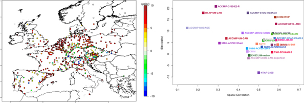
Figure 1. Left : average summertime bias (ppbv) of the 25-model composite over the historical period calculated as by comparing the bilinearly interpolated model value to the measurement site with the observation. Right: average bias (ppbv, y-axis) and spatial correlation (x-axis) of each contributing model.
Download figure:
Standard image High-resolution imageMost of the work included here is based on the climate scenarios used to inform the Third and Fourth Assessment Reports of the IPCC as documented in the Special Report on Emission Scenarios (SRES) [40]. Arranged by increasing level of global warming reached in 2100, these scenarios are: B1, B2, A1B, A2. Some models used the more recent Representative Concentrations Pathways [41], used to inform the IPCC Fifth Assessment Report. These are known as RCP2.6, RCP4.5 and RCP8.5, which yield a radiative forcing of 2.6, 4.5 and 8.5 W m−2 by the end of the 21st century, respectively. There is some similarity between, respectively, RCP4.5 and SRES B1, and RCP8.5 and SRES A2, but RCP2.6 has no real equivalent in the SRES scenarios. Whereas the evolution of short lived climate forcers were taken into account to project future climate, their impact on atmospheric chemistry was ignored in the simulations presented here.
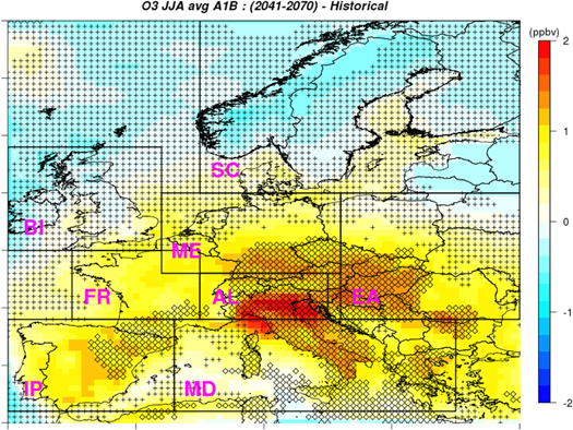
Figure 2. Anomaly of average JJA ozone (ppbv) under the A1B scenario by the middle of the century (2041–2070) according to 9 models for 144 simulated years. At each grid point the shading is the average of the 9 model ensemble, each model response being the average change between future and present conditions (see table 1 for the exact years corresponding to present conditions for each model). A diamond sign (respectively a plus sign) is plotted where the change is significant (respectively not significant) for two-third of the models so that the absence of any symbol indicates the lack of model agreement. Subregions used in figure 3 are displayed on the map with the following labels: AL: Alps—that includes Northern Italy, BI: British Isles, EA: Eastern Europe, FR: France, IP: Iberian Peninsula, MD: Mediterranean, ME: mid-Europe, SC: Scandinavia.
Download figure:
Standard image High-resolution imageResults
Figure 1 shows the map of the ozone climate penalty for the available projections using the A1B scenario, representing total of 144 modelled years. The average of the nine model ensemble is shown. For each model the climate penalty is expressed as the JJA ozone anomaly for the 2041 to 2070 time period compared to historical levels and the significance of the climate penalty is assessed with a student t-test with a 95% confidence level considering each year is independent. The robustness of the climate penalty is subsequently indicated when two-third of the models agree either on the significance of the change, or on its non-significance.
The climate penalty, which is of the order of +1 to +2 ppbv, is robust and statistically significant over large parts of Southern and Central Europe. By the middle of the century, this penalty exceeds +1 ppbv over Spain and Italy. A decrease over the northern British Isles and Scandinavia is found to extend to the north-eastern Atlantic.
Averages of the evolution of the climate penalty for different time horizon across various regions of Europe are given in figure 3. The degree of freedom of boxplots in figure 3 is the number of modelled years for the corresponding scenario and time period. For each year, the anomaly is the difference between JJA average of that year minus the average of JJA values over the historical period for the corresponding model. The distributions include various models and simulated years to capture model spread (although that spread may not capture the full model uncertainty [42]) and inter-annual meteorological variability. The different scenarios are separated in order to acknowledge that they convey an uncertainty of a different nature. However, this approach carries a risk of overweighting models with more simulated years. In order to assess that risk, we also display on the boxplot the median of model averages that are always very close to the median of all modelled years.
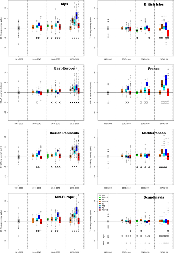
Figure 3. Evolution of summertime (JJA) ozone averages expressed as anomalies compared to the historical period for each model. The boxplots provide the median and upper and lower quartiles of all simulated years in the corresponding 30 year time window as well as whiskers at 1.5 times the inter-quartile distance and points exceeding this value. The median of the average anomaly for each scenario is also given (' + ' sign) to assess the risk of overweighting models with more simulated years by comparison with the median of all simulated years in the boxes. A cross (' × ') is drawn where the signal is statistically different from zero under the same criteria as for the maps in figure 2. Panels are for different geographic regions as indicated in figure 2. The colour-key of scenarios is given in the lower left panel, as well as the total number of models (#mod) and modelled years (#yrs) for each time horizon and scenario.
Download figure:
Standard image High-resolution imageConsidering the whole range of scenarios, we find that the 95% confidence interval of climate penalty on JJA average ozone over all European land surfaces within the latitudes 30 °N and 60 °N and the longitudes 20 °W and 40 °E is [0.44; 0.64] and [0.99; 1.50] ppbv for the 2041–2070 and 2071–2100 time windows, respectively. The impact of climate change on summertime ozone is indeed significant for most scenarios, except for the near future (2011–2040). For the majority of regions and scenarios, climate change acts to increase summertime ozone (AL, EA, FR, IP, MD, ME). This is especially the case for southern, western and central Europe, although decreases are found locally for northern parts such BI and SC, probably in relation with changes in background ozone [10]. The increases are variable in space, time, and across scenarios but remain in the 0–5 ppbv range, except for a few more dramatic increase up to 7.5 ppbv.
For the regions where there is a climate penalty, the magnitude of that penalty tends to broadly increase together with the amount of global warming in the corresponding scenarios. The results obtained with the RCP8.5 constitute a striking exception to that feature where changes are often of a smaller magnitude than for the other scenarios, or even not significant. The more important contribution of global models (many of which show a decline of lower tropospheric ozone [9, 10]) in the ensemble of simulation for the RCP8.5 might play a role here, as discussed further below.
The ozone climate penalty averaged over European land surfaces as a function of the average European surface temperature anomaly is displayed in figure 4. The purpose of this figure is to assess whether the European surface ozone climate penalty can be quantified for a given warming threshold, by comparing various scenarios and time horizons. As before, the ozone climate penalty is the difference of summertime (JJA) mean minus the historical summertime long-term average of the corresponding model. For each model, the penalty by time slices of 10 years is displayed in order to minimize the impact of inter annual variability. The temperature anomaly is computed with respect to the 1971–2000 average. Only CTMs or CCMs driven with GCM boundary conditions corresponding to major coordinated model intercomparison projects are included (CMIP3, CMIP5, ACCMIP) [38, 43, 44].

Figure 4. Summertime average ozone climate penalty over European land areas as a function of the average European surface temperature anomaly (K). Each point is a 10 year average of a given model experiment, colours are for different climate scenarios and symbols for the driving GCM.
Download figure:
Standard image High-resolution image
The ozone climate penalty is again confirmed in the sense that, for this ensemble, the slope of the fit between European ozone and temperature is positive: 0.17 ppbv K−1 but the standard error is high (0.09 ppbv K−1) and the slope cannot be considered as statistically significant with a p-value of 0.056. The correlation is only of 0.24, and ranges over the smaller sub-regions mentioned above from −0.28 (British Isles) to +0.24 (Eastern Europe). This lack of correlation between ozone and average European temperature is likely due to the important role of other meteorological parameters and their interactive effects of surface ozone [17].
Long range transport of ozone is also an important factor as illustrated by the much larger correlation with European mean surface temperature when excluding global (ACCMIP) models (R = 0.59, with a slope of 0.31 ppbv K−1). The variability of the ozone climate penalty simulated over Europe by global models is much larger, to the extent that climate benefits are sometimes shown [10]. This feature can be attributed to the larger role, in global models, of ozone destruction in oceanic low NOx areas induced by the greater availability of OH related to increased water vapour concentrations. This effect might be overestimated in coastal areas compared to regional models because of their coarse resolution, but it is important that regional CTM take into account climate-induced changes in boundary conditions in future assessments [7].
As pointed out above, the impact of climate and land use change on biogenic emissions plays a role on the ozone penalty. We should however note that there are very important uncertainties for this, with a range of a factor of 5 reported for future isoprene emissions across a four-model ensemble [15]. In addition, while most of the models simulate the impact of temperature on biogenic emissions in a dynamical manner, none of them account for the isoprene-inhibiting role of increased CO2 [22].
Conclusion
When aggregated over all European land surface, we find that the increase attributed to climate change on ozone summertime reaches [0.99; 1.50] ppbv by the end of the century. These numbers support the concern that the climate penalty could act against the efforts of mitigation. They are however small compared to the annual rate of ozone change observed since the middle of the 1990s with an order of magnitude of −1 ppbv yr−1 [45, 46]. The studies that explicitly compared the magnitude of projected climate and anthropogenic emission changes all confirmed the larger impact of the later [7, 14, 16, 21]. We thus conclude that even if climate penalty is a reality for ozone pollution, its magnitude compared to recent trends and expected emission projections should not discourage from implementing ambitious mitigation measures.
Acknowledgments
This research was commissioned by the European Environmental Agency through its Topic Centre on Air Quality and Climate Mitigation. It benefited from the support to earlier projects: the European Union's Seventh Framework Programme (FP7/2007-2013) under grant agreements no. 282687 (ATOPICA), no. 282910 (ECLAIRE), no. 247708 (SUDPLAN), no. 282746 (IMPACT2C), no. 037005 (CECILIA); the US Environmental Protection Agency Science to Achieve Results (STAR) Program with simulations done with NOAA, DOE/NERSC and NCSA/UIUC supercomputing resources; SALUTAIR (French Primequal ADEME-MEDDE programme); ACHIA (ADEME) and computing resources of the TGCC/CCRT/CEA; Nordic Council of Ministers (EnsCLIM project no: KoL-10-04); the Swedish EPA through the research programmes CLEO and SCARP, and through the framework of the ERA-ENVHEALTH research programme ACCEPTED; Dutch Knowledge for Climate Programme; the European Union (European Social Fund—ESF) and Greek national funds through the Operational Program 'Education and Lifelong Learning' of the National Strategic Reference Framework (NSRF)—Research Funding Program: Heracleitus II. AUTH acknowledges EGI and HellasGrid for computing resources and technical support. Investing in knowledge society through the European Social Fund. The coordinated ACCMIP and HTAP exercises are also gratefully acknowledged.