
ABSTRACT
Multicolor (BVRI) light curves have been obtained for the newly discovered, 4.21 hr eclipsing dwarf nova RX J0909+1849. The eclipse profiles have been analyzed with a parameter‐fitting model to constrain properties of the system. The model assumes four sources of luminosity: the white dwarf primary star and the secondary star (both assumed to radiate as blackbodies) and an accretion disk characterized as a blackbody whose temperature follows a radial power‐law distribution:T(r) = Td(Rd/r)α, where Td and Rd are the outer disk temperature and radius, respectively. The model also includes an optically thick bright spot at the intersection of the mass transfer stream and the disk periphery. A matrix of model solutions is computed, which covers an extensive range of plausible parameter values. The solution matrix is then explored to determine the optimum values for the fitting parameters and their associated errors.
The mass ratio of RX J0909+1849 is unknown, thus the orbital inclination is not tightly constrained by the model. Five mass ratios have been considered spanning a range of plausible values,0.3≤q(= M2/M1)≤0.7. Over this range of q, the inclination varies between roughly 74° and 80°. Model parameters include the temperatures of the white dwarf (T1) and the secondary star (T2), the radius (Rd ) and temperature (Td ) of the disk periphery, the disk power‐law temperature exponent (α), and the bright spot temperature (Ts ). With the exception of the q = 0.3 models, which required a relatively hot white dwarf (80,000 K), the optimum values of the parameters are nearly constant with mass ratio. For a representative mass ratio of q = 0.5, values of T1 = 26,000 ± 14,000 K,Ts = 18,000 ± 7000 K,Td = 3200 ± 600 K,Rd/RL1 = 0.54 ± 0.08,α = 0.53 ± 0.11, and B−V = 0.45 ± 0.07 are found. A value of T2 = 3400 K has been adopted for all models based on the spectral type of the secondary star (M3–M4).
The observed color (B−V = 0.4 ± 0.2) is consistent with the colors given by the model; thus, it is unlikely that RX J0909+1849 suffers significant interstellar absorption. The observed spectral type of the secondary star suggests an absolute magnitude in the range 10.6<MV(2)<11.0. After correcting the apparent V magnitude at mideclipse by the fraction of light originating from the secondary star (∼94%), a distance of ∼200–250 pc is derived for the RX J0909+1849 system.
Export citation and abstract BibTeX RIS
1. INTRODUCTION
Dwarf novae are a subclass of the cataclysmic variable stars, which consist of a late‐type, near–main‐sequence star (the secondary star) that fills its Roche lobe and transfers gas to a more massive white dwarf companion (the primary star). The transferred gas initially forms a ring surrounding the white dwarf before viscous forces cause the ring to broaden into a disk, allowing accretion onto the white dwarf's surface. Often a conspicuous bright spot is formed at the location where the mass transfer stream impacts the disk. If the mass transfer rate is below a critical value (which depends primarily on the orbital period), then material builds up in the ring until a thermal instability ensues in the disk gas, causing its viscosity to increase precipitously. The result is a significant increase in the mass accretion rate through the disk. Since the disk luminosity is proportional to the mass accretion rate, the disk brightens considerably (typically by 1–3 orders of magnitude, depending on the system), giving rise to a dwarf nova eruption. A thorough overview of cataclysmic variables can be found in Warner (1995).
The physical properties of the binary systems (e.g., orbital inclination, mass ratio, temperatures of the component stars, and the size and radial brightness profile of the accretion disk) can be studied most easily in eclipsing cataclysmic variables where the ingress and egress of the white dwarf and disk from behind the secondary star allow the relative sizes and luminosities of the components to be studied. In the case of the accretion disk component, the eclipse allows emissivity of the gas to be studied as a function of disk radius. Among the cataclysmic variables, dwarf novae provide the best opportunity for studying changes in the structure of the accretion disk that occur in response to a varying mass accretion rate.
As part of a program of identifying cataclysmic variables from the Hamburg‐Schmidt objective prism survey (Hagen et al. 1995), Gänsicke et al. (2000) recently reported the discovery that HS 0907+1902 (=RX J0909.5+184956) is an eclipsing dwarf nova with an orbital period of 4.21 hr. In order to learn more about the physical properties of this system, we obtained multicolor eclipse light curves of RX J0909+1849 in quiescence, approximately 3 weeks after one of its dwarf nova eruptions. Here we present the results of that study.
2. OBSERVATIONS
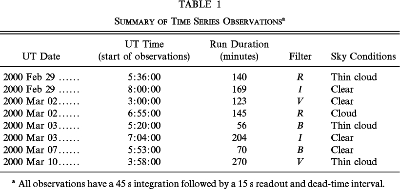
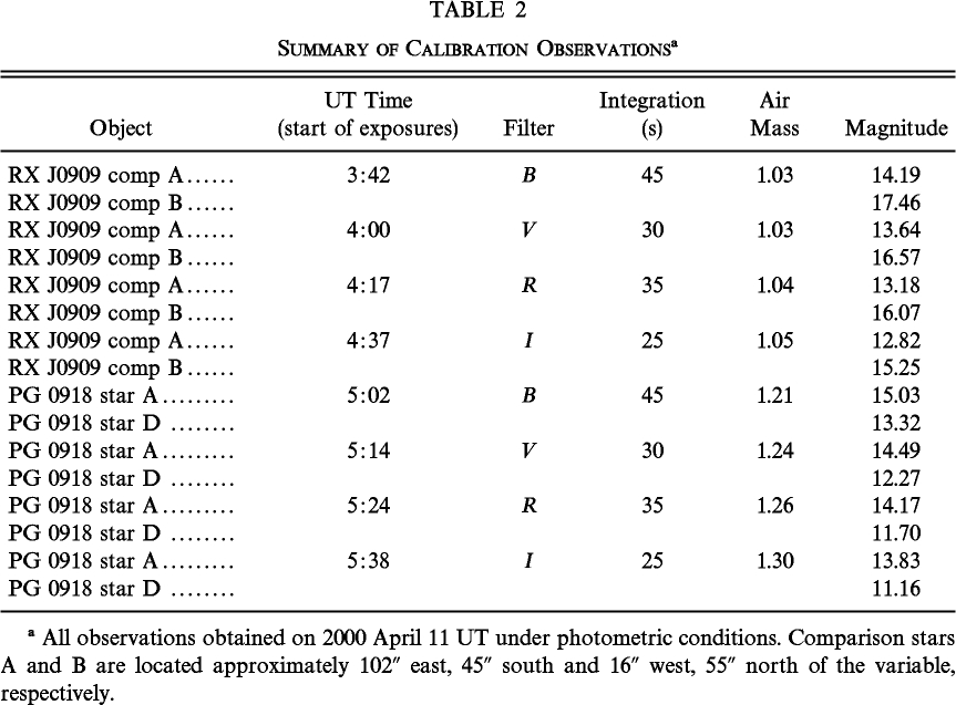
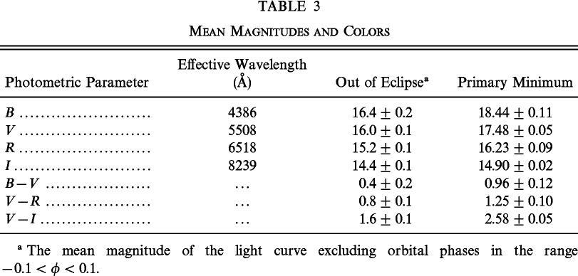
Time‐resolved photometric observations of RX J0909+1849 were obtained during five nights in 2000 February and March using the 1 m reflector at the Mount Laguna Observatory. A summary of our time series observations is given in Table 1. On each night a series of 45 s exposures were taken through either broadband B, V, R, or I filters and imaged on a Loral 20482 CCD. The CCD was read out in a fast photometry mode whereby images of RX J0909+1849 and two comparison stars were recorded simultaneously. To achieve the necessary time resolution and to conserve computer disk space, only a central 4002 subimage of the chip was read out and recorded. The data were debiased and flat‐fielded using standard routines in the Image Reduction and Analysis Facility (IRAF).1 Magnitudes for RX J0909+1849 and the two comparison stars were then determined using the IRAF APPHOT package. Atmospheric extinction variations were removed to first order by dividing the flux of RX J0909+1849 by the brighter of the two comparison stars. The resulting differential light curves were then placed on an absolute scale by calibration of the comparison stars against the standard stars in Landolt (1992). A summary of our calibration observations is given in Table 2. During the five nights of observation, we observed a total of eight eclipses, two in each color. The resulting eclipse light curves are displayed in Figure 1, with the mean photometric parameters given in Table 3.
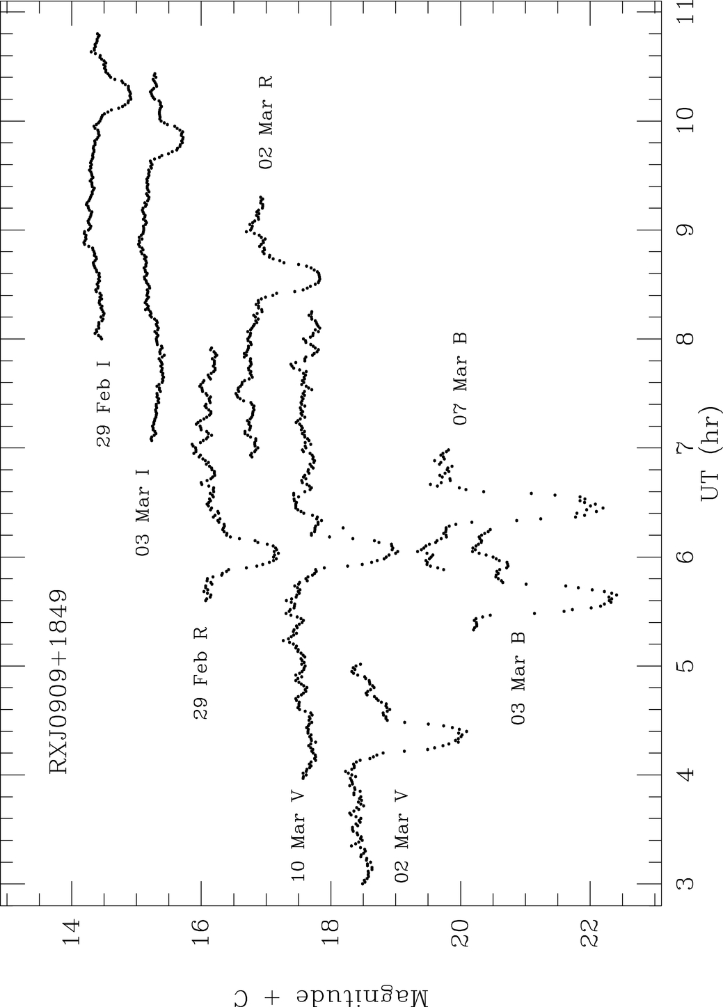
Fig. 1.— Multicolor light curves of RX J0909+1849. For clarity of presentation, the data have been offset downward by addition of the following constants: I March 3, 0.8 mag; R February 29, 1.0 mag; R March 2, 1.5 mag; V March 10, 1.5 mag; V March 2, 2.5 mag; B March 7, 3.5 mag; B March 3, 4.0 mag.
 |
 |
 |
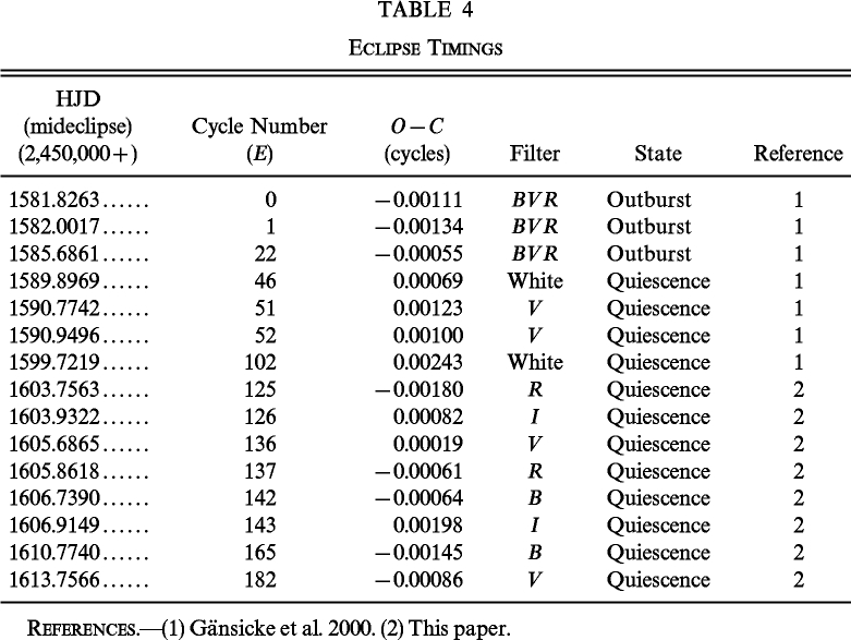
Times of mideclipse were determined by fitting a parabola to the region near the minima of the eclipse profiles. A linear least‐squares fit of the combined times of mideclipse from our study and that of Gänsicke et al. (2000) yields the following eclipse ephemeris:
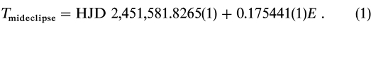
A summary of the eclipse parameters is given in Table 4.
 |
3. ECLIPSE MODELING
To model the RX J0909+1849 system, we use an updated version of the eclipse profile synthesis program developed by Campbell & Shafter (1995). This program, which is based on the parameter‐fitting model of Zhang, Robinson, & Nather (1986) and Zhang & Robinson (1987), decomposes the system luminosity into four components: the white dwarf and secondary star, the accretion disk, and the bright spot where the mass transfer stream impacts the disk. The model light curve is generated from the eclipse by the secondary star of the three remaining sources of radiation. The net flux at a given orbital phase is computed by summing the contribution from the uneclipsed regions of each light source. The model flux for a given color is weighted by the product of the filter transmission and the CCD spectral response appropriate for the particular bandpass. The model fits the normalized light‐curve intensities rather than the calibrated fluxes of the system. In effect we fit only the shapes and depths of the eclipse profiles. Although our model only fits normalized eclipse profiles, it also computes a model B−V color that can be compared with the observed value. To convert the blackbody fluxes computed by the model to an equivalent B−V color, we use the transformations given in Matthews & Sandage (1963).
The model assumes the accretion disk to be flat, circular, optically thick, radiating as a blackbody, and lying in the orbital plane of the system. In addition, the model assumes a power‐law radial temperature profile for the disk (Pringle 1981):

where Td and Rd are the outer disk temperature and radius, respectively, for an optically thick, steady state disk α = 0.75.
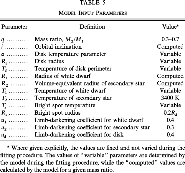
The fluxes of the secondary star and of the white dwarf primary star are computed assuming they are spherical blackbodies of a specified temperature and radius. Since the secondary star is tidally distorted, the spherical approximation will lead to a slight overestimation of its cross‐sectional area (and thus its flux contribution) at mideclipse. The effects of gravity darkening and heating of the inner hemisphere of the secondary star are neglected, since we model only a limited portion of the orbit centered on primary eclipse, when the effects of gravity darkening are minimal and the irradiated hemisphere of the secondary star is obscured from view. A linear limb‐darkening law with the coefficients given in Table 5 was employed when computing the flux from the accretion disk and the photospheres of the primary and secondary stars.
 |
The bright spot is modeled crudely by first considering a circular region of radius 0.20Rd , which lies in the plane of the disk and whose center is located at the point of intersection between the mass transfer stream and the disk perimeter. The bright spot region is then defined by the area of intersection of this circular region and the accretion disk. The spot is assumed to radiate as a blackbody whose temperature varies linearly from a specified peak value, Ts , at the spot center to the local disk temperature at the spot periphery. As in the case of the secondary star, the model assumes a simple isotropic radiation pattern for the bright spot flux, and no attempt is made to model any phase‐dependent flux variation outside eclipse.
3.1. Input Parameters
The model requires that we specify the input parameters listed in Table 5. Since only relative intensities are computed by the model, it is not necessary to specify the distance to the system or to place the dimensions of the system on an absolute scale in order to compute a model light curve. The relevant system dimensions such as the radius of the accretion disk and secondary star can be specified in units of the stellar separation, both of which are functions solely of the mass ratio,q = M2/M1.
Several of the parameters listed in Table 5 can be computed once the mass ratio is specified. The mass ratio and the inclination of the orbit to the plane of the sky, i, are related by the eclipse width (Chanan, Middleditch, & Nelson 1976). For RX J0909+1848 the observed width of the B eclipse at half‐depth yields Δϕ = 0.064. In addition to the orbital inclination, the individual stellar masses and system dimensions also can be determined once the mass ratio is specified. We begin by noting that the effective radius of the Roche lobe–filling secondary star can be expressed as a function of the mass ratio (Eggleton 1983):
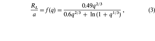
where RL /a is the volume‐equivalent Roche lobe radius in units of the orbital separation and is a function of q alone.
If we assume that the secondary star fills its Roche lobe (R2 = RL) and obeys a power‐law mass‐radius relation of the form
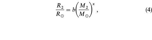
then its mass can be expressed as a function of the orbital period and mass ratio of the system:
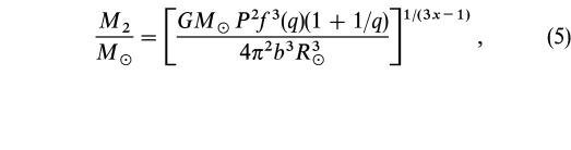
where f(q) is given by equation (3).
Adopting the coefficients b = 0.91 and x = 0.75 from the study of secondary stars in cataclysmic variables by Smith & Dhillon (1998), the mass of the secondary star can be expressed as
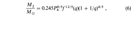
where Ph is the orbital period in hours. The radius of the secondary star then follows from equation (4).
Once the mass of the secondary star is computed, the mass of the white dwarf primary follows immediately for a given mass ratio. The radius of the white dwarf can then be computed using Nauenberg's (1972) derived mass‐radius relationship for an electron degenerate white dwarf:
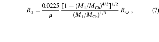
where μ is the mean molecular weight of the star and MCh is the Chandrasekhar mass limit. Adopting μ = 2, we find the following convenient expression for the radius of the primary star:
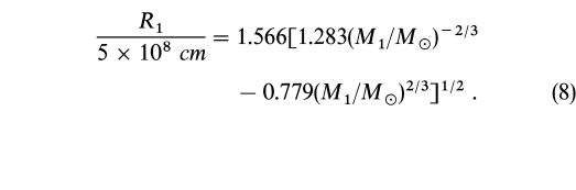
To begin the fitting procedure, the mass ratio must be specified. Unfortunately, the mass ratio for RX J0909+1849 is unknown. We can, however, make a rough estimate of its value. As reviewed by Warner (1995), the dependence of M2 on q is weak, and to a good first approximation the mass of the secondary star can be expressed as a function of the orbital period alone. For a period of 4.21 hr, equation (2.100) of Warner (1995) allows us to make a preliminary estimate that M2≃0.39 M⊙. On the other hand, according to Smith & Dhillon (1998), the average primary mass for 16 cataclysmic variables above the period gap is 0.80 ± 0.22 M⊙. Combining this value with the mass of the secondary star estimated above, the mass ratio of the system is estimated to be ∼0.5. A firm lower limit on the mass ratio, q≃0.3, is found by requiring that M1<MCh = 1.4 M⊙. On the other hand, requiring that mass transfer be stable provides an upper limit to the mass ratio of q = 0.7 for a secondary star of 0.4 M⊙ (Politano 1988). Thus, for the parameter‐fitting analysis, a range of values for q is considered: 0.3, 0.4, 0.5, 0.6, and 0.7, with a value of q = 0.5 representing our best initial estimate.
3.2. Light‐Curve Fitting
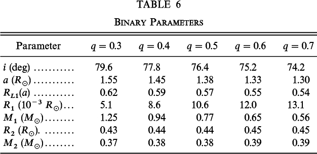
The required input parameters listed in Table 5 can be divided into two groups. The first group consists of parameters whose values are thought to be known a priori and are not varied during the fitting procedure. The second group consists of free parameters whose values we estimate through the fitting procedure. The latter group includes the temperature of the white dwarf, T1, and four accretion disk parameters: the temperature and radius of the disk's periphery, Td and Rd , the bright spot temperature, Ts , and the radial temperature power‐law parameter, α. The orbital inclination and the mass and radius of the white dwarf and secondary star are determined once q is fixed. Table 6 summarizes the values of the binary system parameters computed solely based on the mass ratio and not determined during the fitting procedure.
 |
Without further information, the temperature of the secondary star would have to be included as a free parameter; however, in the case of RX J0909+1849, we can estimate T2 from the observed spectral type. The spectroscopic observations of Gänsicke et al. (2000) suggest that the secondary star has a spectral type between M3 V and M4 V. This value is consistent with that found from equation (4) of Smith & Dhillon (1998), which estimates a spectral type of ∼M3 for the secondary star in a system with an orbital period of 4.21 hr. According to the compilations of Popper (1980), main‐sequence stars with spectral types in this range have effective temperatures between ∼3370 and 3480 K. We have adopted T2 = 3400 K in our model computations.
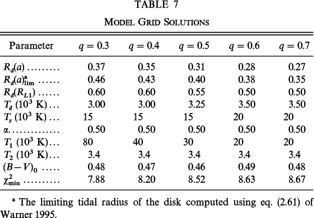
To begin the fitting procedure, we select plausible ranges of values for the five fitting parameters. Then each parameter is varied (one at a time) through a suitable range while the remaining parameters are held constant. In this way a five‐dimensional parameter space of models is explored for plausible solutions. The goodness of fit at each stage is determined using a standard χ2 test. The deviations between the model and the data are determined for each of the four colors, and the final χ2 statistic is determined by weighting each of the colors equally. Since we model the eclipse only, the calculation of χ2 is restricted to orbital phases between ϕ = -0.05 and ϕ = 0.09, which corresponds roughly to the time from the onset of disk ingress to the completion of bright‐spot egress. The entire fitting process was repeated five times, once for each assumed mass ratio. The best‐fitting solutions for our grid of models are given in Table 7.
 |
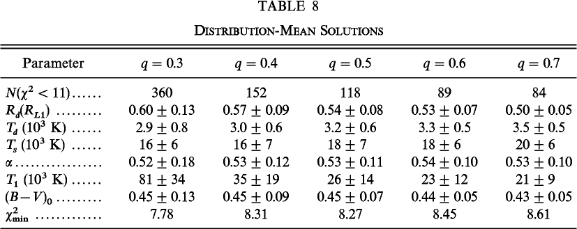
3.3. The Model Solution Distributions
Exploring the matrix of possible solutions reveals that many combinations of parameters produce good fits to the data. The problem is to determine which particular combination of parameters best represents the true model for RX J0909+1849. To assess how well each of the parameters is constrained, we have established a procedure whereby the distribution of acceptable solutions can be explored. In practice, we established an upper limit to the value of χ2 that represented an acceptable fit to the data (taken to be χ2<11) and constructed frequency distributions for each of the fitting parameters. The mean and standard deviations of each parameter distribution are summarized in Table 8, while the frequency distributions for the five free parameters and the model B−V color for representative mass ratios of q = 0.3, 0.5, and 0.7 are shown in Figures 2, 3, and 4. The range over which each parameter is varied has been chosen to be sufficiently large so that all solutions with χ2<11 were explored. For each of the four fitting parameters excluding the white dwarf temperature, a total of nine values provided adequate sampling. For T1 a total of 15 values were necessary to provide adequate sampling while covering the full range of solutions. In all, a total of 98,415 (=94 × 15) models were computed for each mass ratio. For a given value of q, the total number of models with χ2<11 can be found in Table 8. We note that the model solutions are robust in the sense that they do not depend strongly on the value of the cutoff χ2 adopted in the analysis.
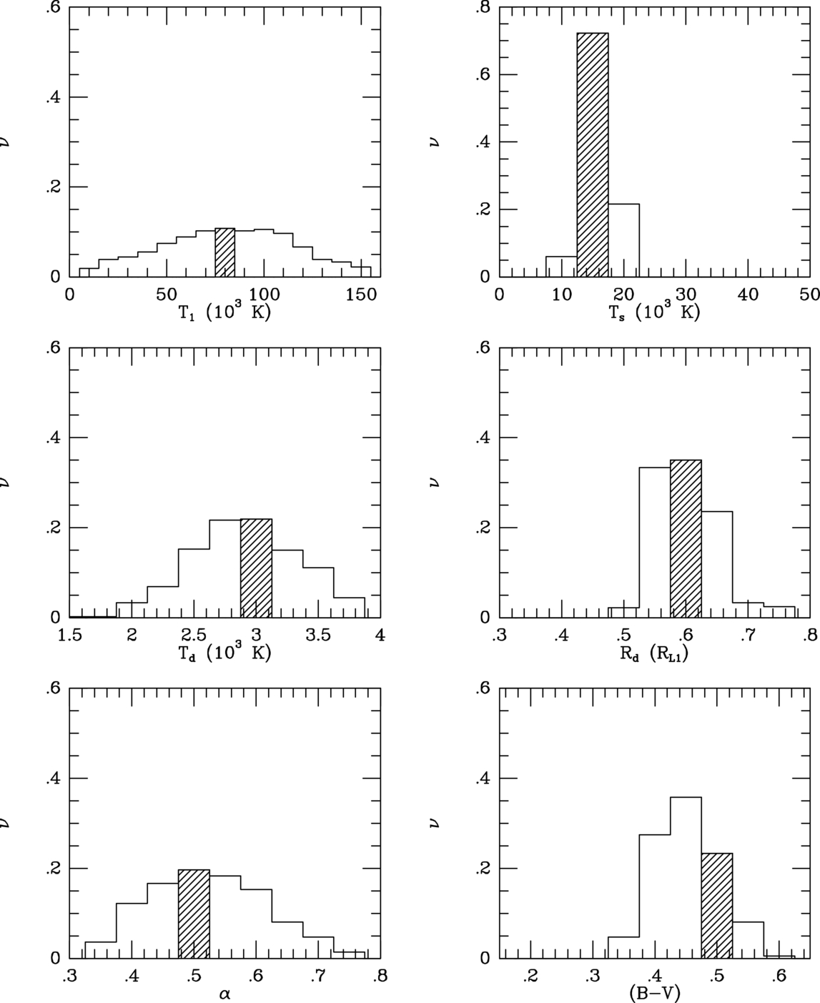
Fig. 2.— q = 0.3 frequency distributions for each variable input parameter. The range of the distribution for each parameter has been chosen to include all combinations of parameters in the grid that resulted in acceptable fits of the model to the data (χ2<11). The hatched regions indicate the values of the grid parameters that produced the optimum fit to the data.
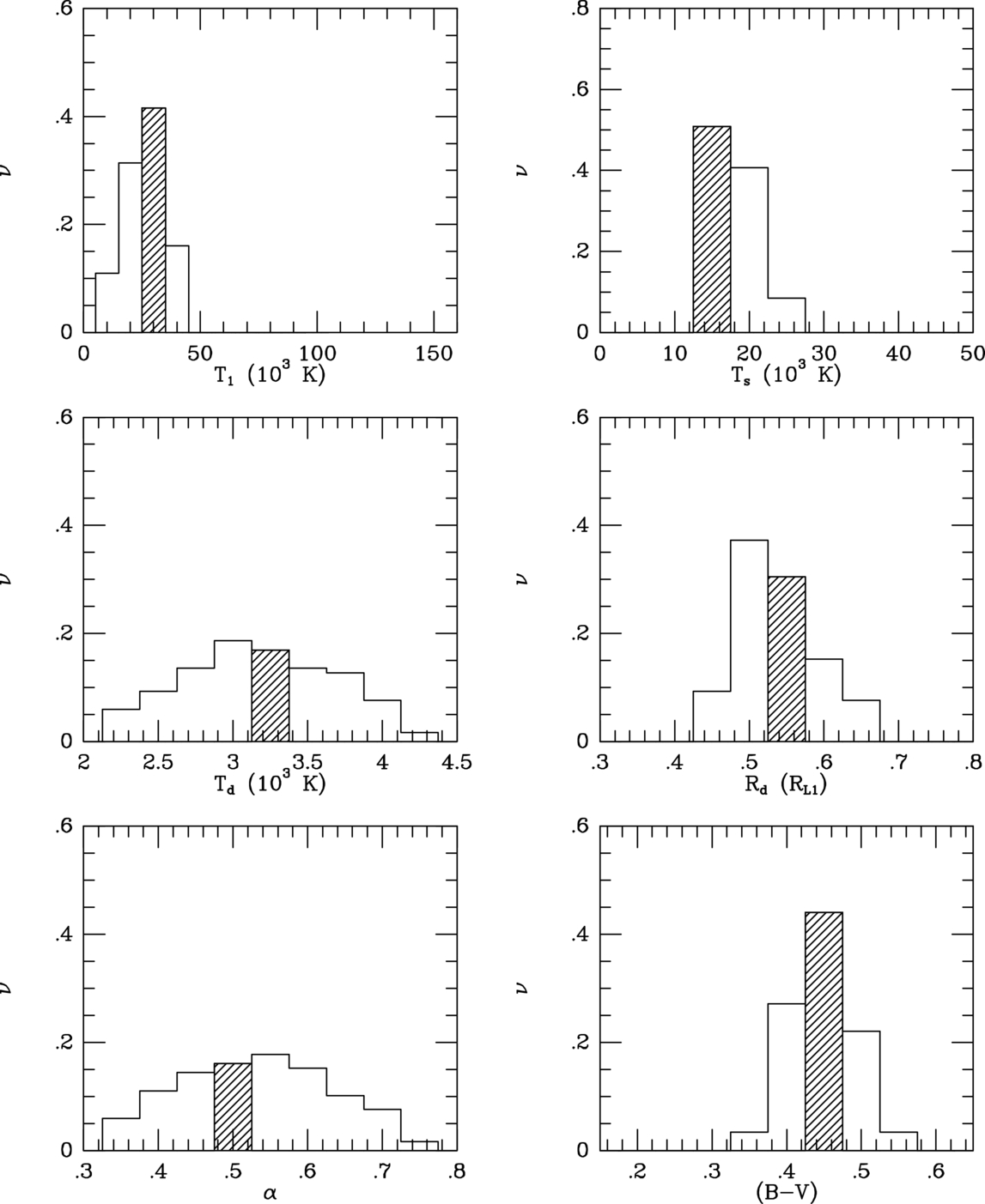
Fig. 3.— Same as Fig. 2, but for q = 0.5
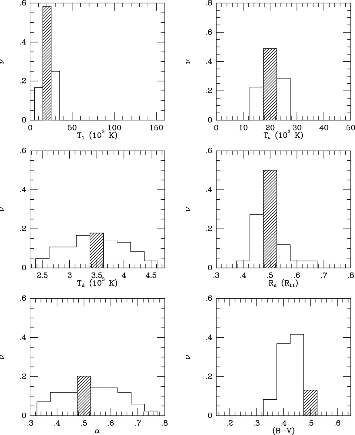
Fig. 4.— Same as Fig. 2, but for q = 0.7
 |
The frequency distributions reveal how well a given parameter is constrained by the model fit. If a parameter is tightly constrained by the data, its frequency distribution will be narrow and centered on its optimum value. Thus, the mean and standard deviation of each distribution provide not only an estimate of the optimum value for a specific parameter but also a quantitative estimate of its uncertainty. The parameters were the most poorly constrained in the q = 0.3 models as evidenced by the larger standard deviations for all parameters, particularly in the case of the white dwarf temperature. For our cutoff χ2<11, solutions were found in the range 10<T1(K)/103<150, while much smaller ranges were found for the other mass ratios. This large range in T1 resulted in the largest number of fits [N(χ2<11) = 360] and the best fit overall (χ2 = 7.88) being generated with a mass ratio, q = 0.3. Nevertheless, close fits were also obtained for the other values of q; thus, we are unable to determine confidently the mass ratio based on our eclipse modeling. Unfortunately, since q is poorly constrained, so is the orbital inclination. On the other hand, the best‐fit values of several other parameters, including the bright spot temperature, Ts , the disk radius, Rd , and most notably, the disk temperature profile parameter, α, are reasonably constant regardless of the assumed value of q, and we therefore consider these parameters to be well constrained by our analysis.
Since the model light curves for the various mass ratios fit the data nearly equally well, we show in Figure 5 only the model light curves for q = 0.5 plotted together with the phased eclipse data. The model light curves fit the observed data quite well, with two exceptions: the I‐band eclipse and the late‐egress portion of all eclipse profiles. We attribute the poor I‐band fit to ellipsoidal variations, which are not included in our model. The late‐egress portion of the eclipse profile corresponds to the egress of the bright spot. Additional light curves will be required to smooth out the stochastic variations (i.e., "flickering") and better define the shape of the bright spot egress. Thus, our model solutions for the bright spot temperature should be considered only as a rough estimate. The poor fit just prior to eclipse is likely the result of flickering and anisotropy in the bright spot radiation, neither of which are included in our model.
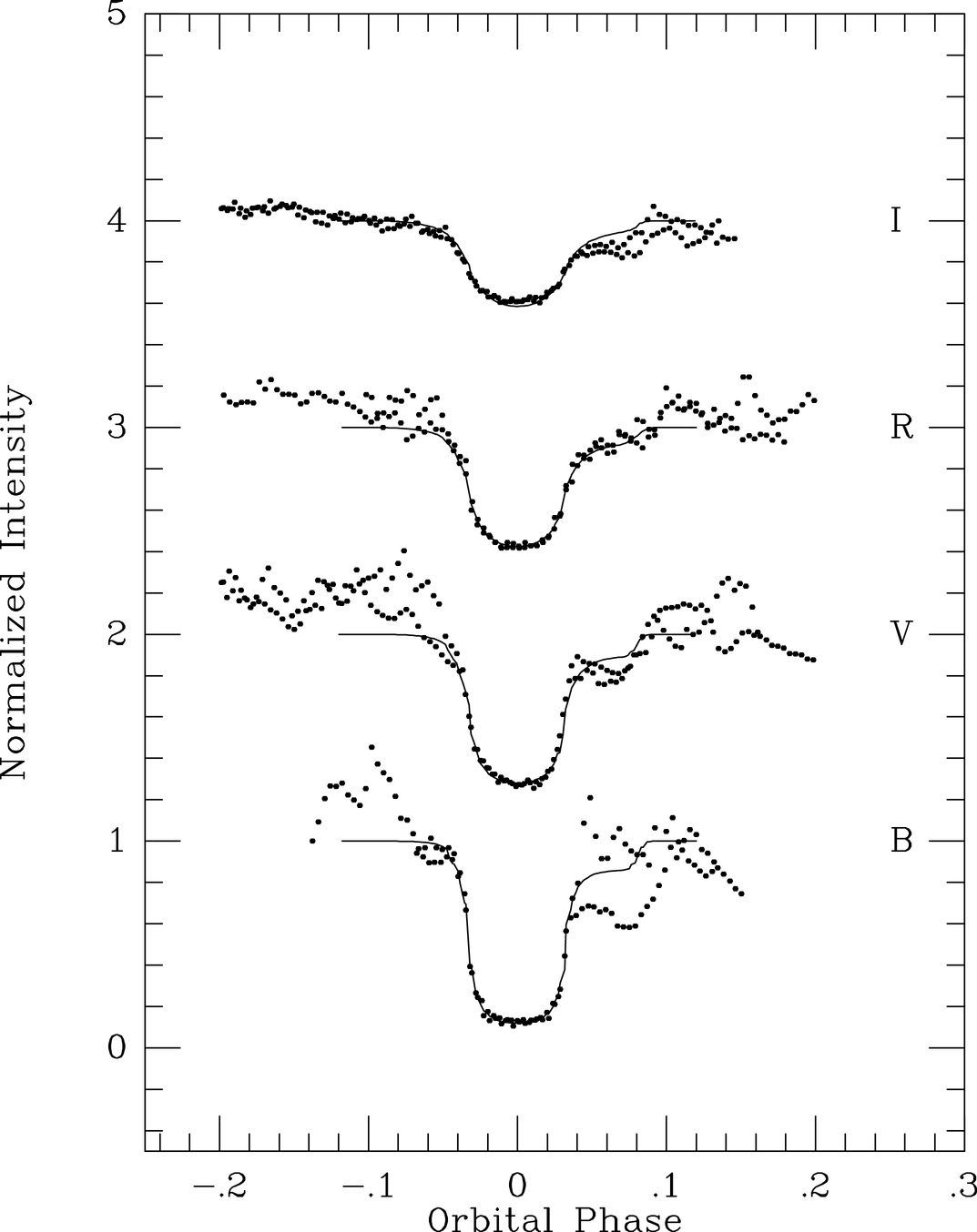
Fig. 5.— Best‐fitting model eclipse profiles (solid lines) for q = 0.5 are plotted together with the observed data. The data have been converted to relative intensity and normalized to unity outside eclipse. For clarity of presentation the V, R, and I data have been shifted upward by constant offsets of 1, 2, and 3, respectively.
3.4. Correlations between Model Parameters
In addition to providing a means for exploring the range of acceptable solutions for a given parameter, the matrix of solutions also allows us to explore possible correlations between model parameters. We begin by considering an expanded set of model solutions defined by χ2<13, where the expanded set of solutions allows for a greater range of parameter values from which to study correlations. We then examine the set of solutions for pairs of parameters defined when the remaining parameters are held constant at their optimum values (Table 8). For a total of five fitting parameters, there are a total of 10 such pairings. Figure 6 illustrates the correlations between these 10 pairs of parameters. The most highly correlated parameters are the accretion disk parameters, Rd , Td , and α, which together determine the disk luminosity. This relationship is not surprising since it is the relative luminosities of the disk and secondary star (whose luminosity is fixed in our models) that determine, to first order, the depth of eclipse. For example, a relatively flat disk temperature profile (small α) can be compensated for to a degree by a higher temperature at the disk periphery (larger Td ), or by a larger disk (larger Rd ), or both. Similarly, for a given α, a lower value of Td would require a larger disk to maintain an acceptable fit to the data.

Fig. 6.— Correlations between pairs of model parameters for q = 0.5 are shown and the correlation coefficient, r, given for each of the 10 possible pairings of the five model parameters. In each case a range of model solutions (χ2<13) for each pair of parameters is plotted, while the remaining three parameters are held fixed at their optimum values (Table 8).
The correlations just described do not provide for a set of equally good fits, however, as second‐order effects related to the detailed eclipse profile come into play. Two of the disk parameters in particular, the outer radius (Rd ) and the power‐law index (α), strongly affect the shape of the eclipse profile. The outer radius of the disk affects the width at the top of the eclipse, particularly at longer wavelengths, while the temperature structure parameter α controls the shape of ingress and egress: the steeper the temperature gradient, the more rounded the eclipse profile. Thus, despite the presence of correlations between some of the input parameters, it is still possible to use the detailed eclipse profiles to constrain the system parameters.
3.5. The Distance to RX J0909+1849
The distance to RX J0909+1849 can be estimated from a comparison of the absolute magnitude of the secondary star, the observed brightness of the system at mideclipse, and an estimate of the interstellar extinction along the line of sight. The latter quantity may be estimated from a comparison of the observed and model B−V colors. RX J0909+1849 has an observed B−V color of 0.4 ± 0.2 outside of eclipse, where much of the uncertainty is due to the limited phase coverage of our B‐band data outside eclipse. To within the observational errors, the observed color is consistent with the value of B−V = 0.45 ± 0.07 given by the best‐fitting model. In the absence of any observed reddening, we assume AV = 0 along the line of sight to RX J0909+1849.
The absolute magnitude of the secondary star can be estimated from the compilations of the radiative parameters of lower main‐sequence stars by Popper (1980). For a secondary star of radius R2 = 0.44 R⊙ and spectral type M3 V–M4 V, we find 10.6<MV(2)<11.0. According to our best‐fitting models, the secondary star contributes approximately 94% of the V‐band light at mideclipse. At mideclipse V = 17.48 ± 0.05, so we estimate that V(2) = 17.55 ± 0.05. Given the range of MV found above and adopting AV = 0, we estimate that RX J0909+1849 lies at a distance roughly in the range of 200–250 pc. This value is consistent with the value of 320 ± 100 pc estimated by Gänsicke (2000).
3.6. Comparison with Similar Systems
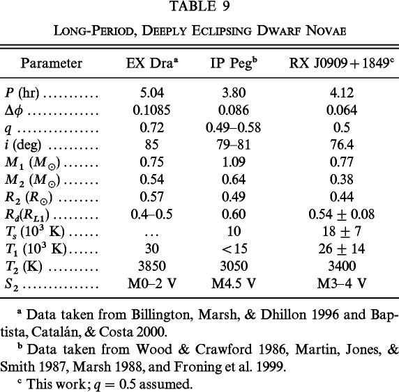
Deeply eclipsing dwarf novae offer the best opportunity to determine the fundamental properties of cataclysmic variables. The vast majority of such systems are found below the period gap and are members of the SU UMa class of dwarf novae. Above the gap there are a total of six eclipsing dwarf novae: EM Cyg (P = 6.98 hr; Beuermann & Pakull 1984), EX Dra (P = 5.04 hr; Fiedler, Barwig, & Mantel 1997), BD Pav (P = 4.30 hr; Barwig & Schoembs 1983), U Gem (P = 4.25 hr; Smak 1993), IP Peg (P = 3.80 hr; Wolf et al. 1993), and now RX J0909+1849. Of these six dwarf novae only three are deeply eclipsing (i.e., the white dwarf is eclipsed): EX Dra, IP Peg, and RX J0909+1848. Table 9 shows a comparison between the parameters for each system. Although most parameters are not well determined, the available evidence suggests that the systems are quite similar. The longest period system, EX Dra, appears to have the highest orbital inclination (i = 85°) and the largest mass ratio (q = 0.72). On the other hand, available evidence suggests that IP Peg and RX J0909+1849 are quite similar. One notable, qualitative distinction between the two systems is that IP Peg displays a much more prominent pre‐eclipse "hump" in its light curve compared with RX J0909+1849. A plausible speculation is that the accretion disk or the secondary star is brighter than its counterpart in IP Peg, thus making the bright spot in RX J0909+1849 less conspicuous. Indeed, at the time of our observations RX J0909+1849 had undergone a recent eruption, and it is possible that the accretion disk had not yet completely returned to its quiescent state by that time.
 |
4. CONCLUSIONS
We have presented a first attempt to analyze multicolor light curves and derive system parameters for RX J0909+1849, a newly identified, deeply eclipsing dwarf nova with an orbital period of 4.21 hr. The results of our model fits are summarized in Tables 6–8.
The principal conclusions can be summarized as follows:
- 1.The accretion disk extends to a radius of 0.5–0.6RL1, depending on q, and is characterized by a power‐law temperature parameter, α≃0.5, which is significantly flatter than the α = 0.75 optically thick case.
- 2.Based on the similarity of the observed and the model B−V color, we find no evidence that RX J0909+1849 suffers significant interstellar extinction.
- 3.The observed spectral type of the secondary star (M3 V–M4 V; Gänsicke et al. 2000) implies an absolute magnitude in the range 10.6<MV(2)<11.0.
- 4.The eclipse models reveal that ∼94% of the V light at mideclipse originates from the secondary star. The resulting value of V(2) = 17.55 ± 0.05 suggests that RX J0909+1849 lies at a distance in the range of 200–250 pc.
- 5.Our results suggest that RX J0909+1849 is similar in many respects to the well‐studied dwarf nova IP Peg. One qualitative difference is that the bright spot in RX J0909+1849 does not appear to contribute as strongly to the quiescent light curve. Future observations of RX J0909+1849 at different times during its eruption cycle will be required to establish the extent of the similarity between these two important systems.
Finally, as a general note, given that various combinations of parameters may produce acceptable fits, we recommend that parameter distributions and mean‐distribution solutions be computed when applying parameter‐fitting eclipse models to cataclysmic variable data.
A. W. S. acknowledges support from NSF grant AST 97‐31641. We are grateful to E. L. Sandquist and to the SDSU Computational Science Research Center for computer support made possible through hardware donations from Compaq Computer Corporation.
Footnotes
- 1
IRAF is distributed by National Optical Astronomy Observatories, operated by AURA, Inc., under contract with the National Science Foundation.