
Abstract
Quantum state preparation is a vital routine in many quantum algorithms, including solution of linear systems of equations, Monte Carlo simulations, quantum sampling, and machine learning. However, to date, there is no established framework of encoding classical data into gate-based quantum devices. In this work, we propose a method for the encoding of vectors obtained by sampling analytical functions into quantum circuits that features polynomial runtime with respect to the number of qubits and provides  accuracy, which is better than a state-of-the-art two-qubit gate fidelity. We employ hardware-efficient variational quantum circuits, which are simulated using tensor networks, and matrix product state representation of vectors. In order to tune variational gates, we utilize Riemannian optimization incorporating auto-gradient calculation. Besides, we propose a 'cut once, measure twice' method, which allows us to avoid barren plateaus during gates' update, benchmarking it up to 100-qubit circuits. Remarkably, any vectors that feature low-rank structure—not limited by analytical functions—can be encoded using the presented approach. Our method can be easily implemented on modern quantum hardware, and facilitates the use of the hybrid-quantum computing architectures.
Export citation and abstract BibTeX RIS

Original content from this work may be used under the terms of the Creative Commons Attribution 4.0 license. Any further distribution of this work must maintain attribution to the author(s) and the title of the work, journal citation and DOI.
1. Introduction
Quantum state preparation is a key subroutine in the overwhelming majority of quantum algorithms. Such algorithms as quantum linear system solvers [1–5], quantum Monte-Carlo [6, 7], quantum machine learning [8–10], and general variational quantum approaches [11] require fast and accurate encoding of classical data into quantum circuits. The state preparation subroutine is often considered the main bottleneck limiting the performance of quantum algorithms [9, 12, 13].
In order to prepare a generic n-qubit quantum state, a circuit with depth  is required since all 2n
inherent parameters corresponding to amplitudes must be encoded using different gates [14]. However, the depth can be reduced to
is required since all 2n
inherent parameters corresponding to amplitudes must be encoded using different gates [14]. However, the depth can be reduced to  by using
  ancillary qubits [15]. Those approaches do not solve the problem of exponential circuit growth with increasing the number of coding qubits and are impractical for large n, especially in case of noisy intermediate-scale quantum (NISQ) devices with finite fidelity and limited connectivity [16]. On the other hand, one can slightly decrease the circuit depth in exchange for an approximation error [17] using, for instance, the entanglement reduction technique [18]—specific classes of quantum states, e.g. normal distributions, can be prepared utilizing relatively shallow circuits [19], however, such methods still suffer from an exponential circuit width and a complex gate realization.
General engineering of quantum circuits specifically for the generation of particular states is challenging and impractical. On the other hand, variational quantum circuits with fixed ansatz, which serves as a general state engineering tool [11], provide a promising approach to state preparation. The general class of quantum states that can be efficiently prepared via variational circuits using classical computations is Hierarchical tensor formats [20]—only such states allow for the contraction with a variational circuit in linear time with respect to the number of qubits [21–23]. Here, we focus on one of the most well-studied and straightforward tensor formats, the matrix product states (MPSs) [21, 22, 24], which is at the core of a variety of tensor networks algorithms [25–27]. In contrast to existing MPS-based algorithms for quantum state preparation, our work contributes three novel aspects:
- We mainly focus on the encoding of vectors obtained by sampling analytical functions, since they are of the most interest for quantum practical applications, including partial differential equations [28, 29], two-electron integral calculation [30], sampling tasks [31], calculation of expectation values [6], which is required e.g. in finance [12];
- We introduce and utilize the Riemannian optimization for the update of quantum gates, which allows us to avoid spurious maxima of the fidelity and achieve higher accuracy and speed;
- We develop a scheme, which is resistant to barren plateaus [32], and numerically verify the robustness up to 100 qubits using QMware system (see appendix
A ).
1.1. Comparison with previous works
The matrix product state formalism, which emerged from the description of many-body quantum systems [21, 24], can be utilized for efficient quantum state preparation [33–35]. Although such methods are accurate, they require unitary operations acting immediately on the  qubits, where r is a rank (bond dimension) of the corresponding MPS [24], which is undesirable for modern quantum computers considering the limited connectivity and high gate errors. To reduce the hardware requirements, a matrix product disentangler algorithm was developed in [36], which prepares the state approximately and requires the implementation only of two-qubit gates acting on neighbor qubits. The disadvantage of this algorithm is that updating the gate parameters occurs sequentially layer-by-layer, and not on all gates simultaneously, which causes a higher approximation error [37]. Also, the quantum circuit is fixed and cannot be tuned accordingly to the given quantum hardware topology.
To facilitate the change in the architecture of the quantum circuit and simultaneously optimize all the gates in it, a projected gradient descent algorithm based on the automatic differentiation [38] was introduced in [37]. Firstly, the approximation error is minimized over unconstrained latent gates in a general matrix space, which are automatically differentiable. Secondly, the polar decomposition is applied to each latent gate independently to turn it into the actual (unitary) gate. However, the latter step is not variational, i.e. it does not take into account the gradient direction, and may produce a suboptimal solution.
In this work, we use a more natural update procedure for variational circuits aimed at MPS preparation based on the Riemannian optimization [39], where the gates are updated within the manifold of unitary matrices (see appendix
2. Results
2.1. The protocol idea—reducing everything to tensors
The matrix product state is a compressed representation of a vector that was originally introduced to approximate the ground state of a many-body Hamiltonian in quantum theory. The main characteristic of such a representation is the rank (bond dimension) r, which expresses the correlations and entanglement of the state vector. In fact, using singular value decomposition (SVD) [43] or cross-approximation [44], any 2n
vector can be represented as MPS with the number of elements  . In the worst scenario, the rank r depends exponentially on n. However, considering vectors arising from sampling of analytical functions on an discretized interval, often a small and n-independent rank is sufficient to approximate the function with high accuracy [41]. Moreover, there is an exact MPS-decomposition for trigonometric, exponential, polynomial and rational functions [45]. That is why the idea outlined in this work is not to consider the preparation of arbitrary states, but vectors that can be represented as MPS with a small rank. It is important to note that the set of such states, although it may seem small, nevertheless covers a wide range of the applied problems (see Appendix
The key quality of the MPS is weak entanglement. Indeed, considering the entropy of the reduced subsystem ![$\rho = Tr_2{[\vert \psi\rangle \langle \psi\vert]}$](https://content.cld.iop.org/journals/2058-9565/8/3/035027/revision2/qstacd9e7ieqn9.gif) of an MPS
of an MPS  with rank r, the following bound on entropy
  holds:
  [21]. Since such states feature a small rank, hence weak entanglement, we expect that they can be efficiently approximated by a circuit where only neighbor qubits are coupled and the depth is restricted. Such circuits possess limited entanglement and are similar to circuits specifically generating states belonging to the MPS class [34, 42].
In order to perform the MPS approximation using a quantum circuit, we represent the quantum circuit also as a tensor network allowing us to optimize the gate parameters by processing tensors directly. Leveraging the locality of operations in hardware-efficient circuits, we apply the tensor networks method for circuit simulation and optimization [46, 47]. Such a method allows us to process the circuit with polynomial runtime scaling in the number of qubits.
We emphasize that the learning of the circuit parameters for the state preparation does not need to be run on quantum hardware—the parameters can be learned using tensor networks on a classical computer, which are subsequently embedded in a circuit executed on a quantum processor.
2.2. Encoding and learning
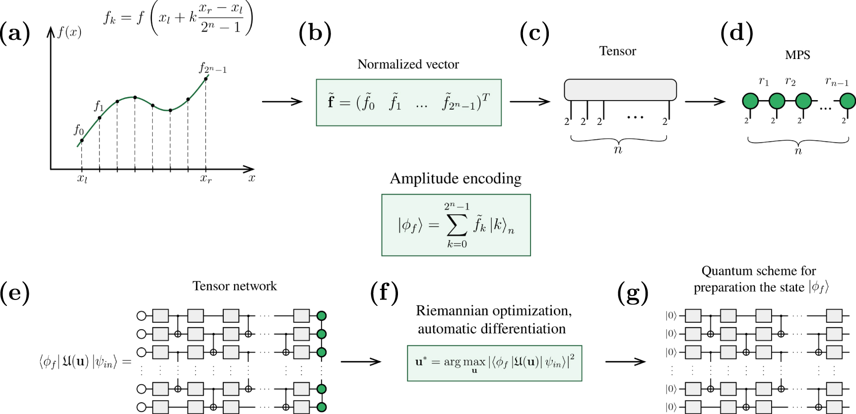
Here, we provide a step-by-step description of the protocol, which is depicted in figure 1. In order to prepare a quantum state  we utilize a variational circuit, which is represented as an action of a variational unitary
  over a state
  . The problem of quantum state preparation is finding a set of parameters a such that the output state
  approximates the desired
  :
:


Figure 1. Overall quantum state preparation scheme. (a) The function to be prepared is sampled in 2n
points on the interval ![$[x_l,\, x_r]$](https://content.cld.iop.org/journals/2058-9565/8/3/035027/revision2/qstacd9e7ieqn7.gif) —a vector of function values is obtained. (b) This vector is normalized and (c) reshaped into a tensor. (d) This tensor is converted into an MPS with visible index dimension equal to 2, and ranks (bond dimensions) equal to ri
[21]. The rank of the MPS is
—a vector of function values is obtained. (b) This vector is normalized and (c) reshaped into a tensor. (d) This tensor is converted into an MPS with visible index dimension equal to 2, and ranks (bond dimensions) equal to ri
[21]. The rank of the MPS is  . (e) A variational n-qubits quantum circuit with neighborhood interactions is represented as a tensor network and then contracted with the MPS to obtain the value of projection of the output quantum state onto the target one (1). (f) The optimal gates of the variational circuit are found using Riemannian optimization and automatic differentiation, yielding (g) the output state as close to the target one as possible.
Download figure:
Standard image High-resolution image2.2.1. Approximation of a function by an MPS: steps (a) to (d)
The desired state  is produced from an analytical function f(x), which is assumed to have a small MPS rank. One way to encode a function into a quantum state is the amplitude encoding. The function is sampled on a given interval
 ![$[x_l, \hspace{3pt} x_r]$](https://content.cld.iop.org/journals/2058-9565/8/3/035027/revision2/qstacd9e7ieqn19.gif) at 2n
equispaced points
at 2n
equispaced points  . Then a normalized vector of function values at these points is encoded in the quantum state amplitudes:
Further, we represent the obtained normalized vector  in the MPS format. For this, the vector is reshaped into a tensor of an order n and then sequential SVD applications allow us to represent it as an MPS [21, 48, 49]. However, the disadvantage of this approach is that it requires 2n
function calls, which is impractical in case of large vectors. Alternatively, the tensor-train cross approximation technique [44] allows one to recover an MPS by an adaptive sampling of just
in the MPS format. For this, the vector is reshaped into a tensor of an order n and then sequential SVD applications allow us to represent it as an MPS [21, 48, 49]. However, the disadvantage of this approach is that it requires 2n
function calls, which is impractical in case of large vectors. Alternatively, the tensor-train cross approximation technique [44] allows one to recover an MPS by an adaptive sampling of just  points. In this work, we utilize the cross approximation algorithm.
2.2.2. Processing a circuit as a tensor network: step (e)
In order to prepare states using NISQ devices we consider a unitary  consisting of sequentially applied single-qubit variational gates
  mixed with CNOTs, as shown in figure 2.

Figure 2. The variational quantum circuit used in all presented experiments. The unitary  is expressed as a product of L unitaries
  sequentially acting on an input state. Each unitary Ul
is a sequence of non-parametric CNOT gates and variational gates
sequentially acting on an input state. Each unitary Ul
is a sequence of non-parametric CNOT gates and variational gates  .
.
Download figure:
Standard image High-resolution imageAs we mentioned in the previous section, the quantum circuit itself should be represented as a tensor network, with gates acting as tensors. The projection of the desired state on the state generated by this circuit  is equivalent to the contraction of two tensor networks:
  as an MPS and utilized circuit as a tensor network. Weak entanglement in shallow circuits with fixed depth, considered here, leads to the linear scaling of the simulation runtime with respect to the number of qubits. To achieve this, we utilize hyper-optimized tensor network contraction introduced in [46] that allows us to find a near-optimal contraction sequence. We show the numerical runtime of the projection of a random MPS
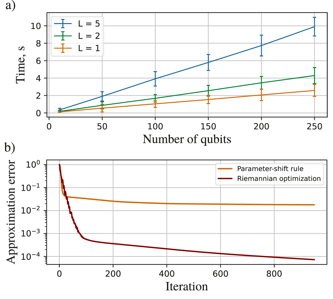
  with rank 2 onto a quantum circuit with different number of layers up to 300 qubits in figure 3(a).

Figure 3. (a) Runtime of a single objective function calculation for varying numbers of qubits for 1-, 2-, and 5-layer circuit. The objective function equation (1) is computed as a tensor network contraction of a quantum circuit with the given number of layers and qubits and an MPS with rank 2, both populated with random parameters. Times are averaged over 100 runs of objective function calculation. (b) The approximation error obtained during an objective function minimization using the parameter-shift rule and the Riemannian optimization. Comparison between mentioned methods is done for a circuit containing 5 qubits and 2 layers approximating a random MPS with rank 2 sampled at 32 points. Since the Riemannian optimization provides a significantly lower error we focus on this method hereinafter.
Download figure:
Standard image High-resolution image2.2.3. Optimization of the quantum circuit: step (f)
One of the most commonly used ways to solve the optimization problem equation (1) is to use the gradient-based parameter-shift rule [50]. Usually in that case, variational gates  depend on the parameters
  and have the form of
  , with σ being a Pauli operator. However, such a direct optimization of
  may suffer from a barren plateau of vanishing gradients due to the nonlinearity of the exponential function.
A more general initial circuit can be constructed from arbitrary unitary operators as variational gates. For this purpose, the Riemannian optimization on the Stiefel manifold of  isometric matrices
  can be used [51], where
  in case of single-qubit gates.
In order to compare those methods, we optimize a 5-qubit circuit with 2 layers of the said structure for preparing a random MPS with rank 2 and show how the approximation error decreases with the number of iterations of gradient descent in figure 3(b). The shift rule achieves only an approximation error worse than 10−2, while the Riemannian optimization provides an error below 10−4. Since the Riemannian optimization provides a better accuracy compared to the parameter-shift rule, we proceed with using the former.
For convenience, let us reformulate the fidelity maximization problem equation (1) into a minimization problem of infidelity (or approximation error)

for a unitary  matrix
  for each
  and
and  . In order to find a local minimum of some differentiable function
  , where
  is
is  isometric matrix, the gradient descent algorithm can be applied

where  is a matrix
  on step t, and α is a step size. Here, we consider the case of single unitary matrix dependence, however this analysis is valid in case of Cartesian product of such matricies [51].
The optimization problem in equation (2) must be constrained to  . This prevents us from using a conventional gradient descent algorithm—we cannot guarantee
  even if
  . Addressing this issue, we use the Riemannian gradient and a retraction R on the manifold [51]. Firstly, instead of a standard gradient
  we use the Riemannian gradient
  which is a vector in the tangent space to the point
  . The construction of a Riemannian gradient
  as an orthogonal projection of the Euclidean gradient
  onto the tangent space is described in the appendix
  is determined by the SVD-retraction

The SVD-retraction is defined as  after computing the SVD
  . By definition, this is just a projection of the matrix
  onto the manifold of
  isometric matrices. Using the retraction instead of a linear step equation (3) allows for the movement along the manifold in a desired direction, satisfying the constraint
  automatically for each step t.
Throughout the optimization, we calculate derivatives of the function with respect to gates using the automatic differentiation technique [38]. While for large and complex networks an analytical differentiation becomes impractical, the automatic differentiation computes derivatives of tensor network programs efficiently with machine precision, in contrast to numerical differentiation. The automatic differentiation, being usually applied for computer programs, is also applicable for tensor networks since the contraction of a tensor network can be represented as a computational graph [52]. Its algorithmic complexity is theoretically guaranteed to be not greater than the algorithmic complexity of the original program, which is equivalent to the complexity of a tensor network contraction [52].
Ultimately, optimization produces a set of unitary matrices that minimize  . Such matrices define single-qubit gates in a quantum circuit for the approximation of the desired state.
2.3. Numerical simulations
In order to demonstrate the capabilities of our method, we consider the frequently-used analytical functions from different classes and prepare them in a many-qubit quantum state. In this work, we consider the polynomial x5, the power function  , the trigonometric function
  , and the Gaussian probability density function. Polynomials and trigonometric functions are often encountered when considering partial differential equations [28] and two-electron integral calculation [30]. Distribution functions are needed for sampling tasks [31] and the calculation of expectation values [6], which is necessary, e.g. in finance [12]. We sample the function over N points on an equidistant grid in
 ![$ [0,1] $](https://content.cld.iop.org/journals/2058-9565/8/3/035027/revision2/qstacd9e7ieqn67.gif) interval and form the function values in a N-dimensional vector, which we approximate using N amplitudes of
interval and form the function values in a N-dimensional vector, which we approximate using N amplitudes of  -qubit state.
In figure 4(a), we show the runtime of the whole state preparation routine as a function of the number of qubits. Here, we set the fidelity to  and the number of layers to 3, which is sufficient to approximate the considered vectors having low MPS ranks (also depicted in figure 4(a)). For all studied functions, our quantum state preparation protocol features a polylogarithmic scaling in the function discretization accuracy: the runtime scales as
  . The number of layers can be increased which leads to an improvement in the approximation error—the infidelity decrease with the number of layers increase is presented in figure 4(b) for a 20-qubit circuit. The runtime breakdown is shown in figure 4(c). As an example, the approximation of a Gaussian density function sampled over 1024 points is depicted in figure 4(d), where a 10-qubit circuit with 3 layers was used to achieve a
  fidelity.

Figure 4. Results on runtime and approximation error for quantum state preparation using MPS formalism. (a) Runtime of our algorithm for the quantum circuit with 3 layers to prepare functions with 10−2 approximation error with respect to the number of qubits. Linear growth in the log–log scale indicates that the preparation is done in a polynomial time. Here, we do not perform simulations with larger circuits, since  points are enough for the one-dimensional function discretization. (b) Approximation error of the function approximation for different number of layers for 20 qubits and a fixed number of optimization iterations equal to 500. Overall, the deeper is the circuit, the higher is the approximation accuracy, however, starting from 5 layers, we observe a stagnation in the accuracy. (c) Runtimes needed to convert a function into MPS (orange) and to perform a single iteration of the circuit optimization (to contract tensor network (circuit simulation) in green and to perform a single iteration of the Riemannian optimization in blue). The approximation accuracy depends on the chosen number of iterations. The runtime features a linear scaling in the number of qubits. The number of layers in all numerical simulations is set to 3. (d) Exact Gaussian density function
  and its approximation with an error
  obtained after 500 iterations of the algorithm using 10 qubits and 3 layers.
Download figure:
Standard image High-resolution imageThe most significant advantage of our method is the ability to achieve a low approximation error using a shallow circuit. While deeper circuits with more parameters improve the accuracy, as shown in figure 4(b), a low error of 0.01%–0.1% can be achieved using only 5 layers. Such an error is of the same order of magnitude as an error of state-of-the-art single two-qubit gates [53].
3. Discussion
3.1. Scaling analysis
Here, we analyze the complexity of the whole algorithm.
In order to investigate how the rank of MPS affects the approximation of our algorithm, we consider a  function specified on an interval
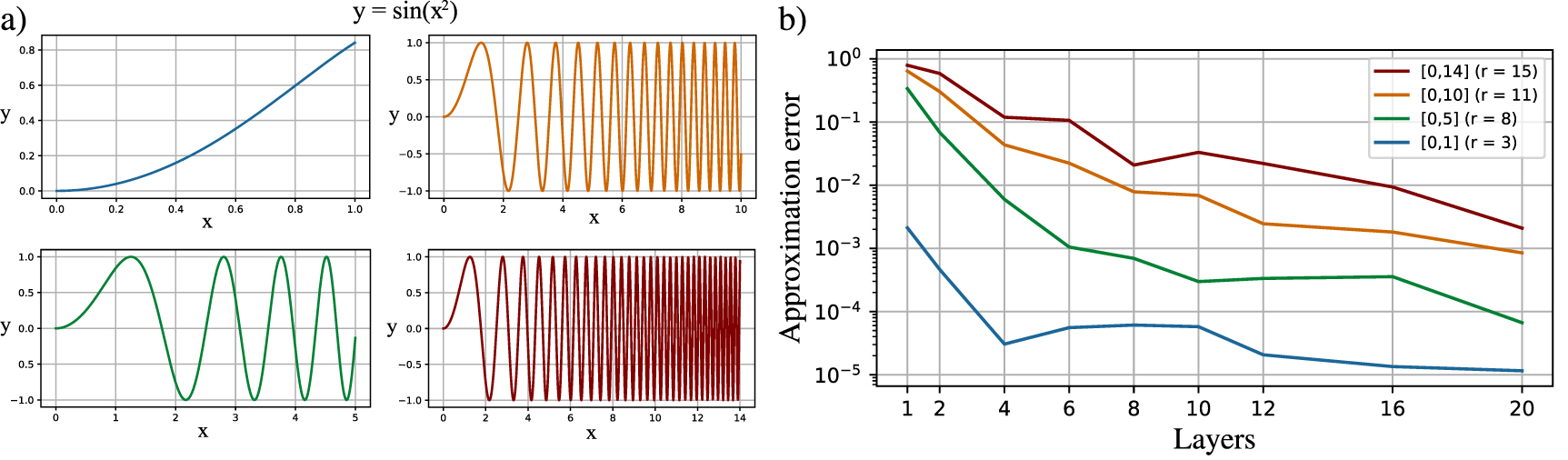
 ![$[0, b]$](https://content.cld.iop.org/journals/2058-9565/8/3/035027/revision2/qstacd9e7ieqn75.gif) . As b increases, the function features faster oscillations and becomes more complex, as shown in figure 5(a), which leads to an increase of MPS ranks. In figure 5(b), we plot the approximation error for various intervals and number of layers. As expected, larger rank requires more layers and the error is larger for a given number of layers for higher ranks. As our goal is to approximate a function, we can fix the number of layers that provides certain accuracy. Generally, it is challenging to specify the exact number of layers for a given approximation as it strongly depends on the approximated function. Practically, for the functions investigated above shallow circuits are sufficient to provide decent accuracy.
. As b increases, the function features faster oscillations and becomes more complex, as shown in figure 5(a), which leads to an increase of MPS ranks. In figure 5(b), we plot the approximation error for various intervals and number of layers. As expected, larger rank requires more layers and the error is larger for a given number of layers for higher ranks. As our goal is to approximate a function, we can fix the number of layers that provides certain accuracy. Generally, it is challenging to specify the exact number of layers for a given approximation as it strongly depends on the approximated function. Practically, for the functions investigated above shallow circuits are sufficient to provide decent accuracy.

Figure 5. (a) Function  shown over four different intervals. As the interval increases, the function shows faster oscillations, which leads to an increase in its MPS rank. (b) Dependence of the approximation error of
  via 10 qubits (1024 grid points) on the number of layers of the quantum circuit for different intervals. Corresponding ranks are shown in parentheses. As expected, with a larger interval (higher rank), more layers are needed to approximate the function.
Download figure:
Standard image High-resolution imageWith fixed number of layers  , the remaining parameters are the number of qubits n and the MPS rank r, which we assume to be restricted, i.e.
  . Each step of the algorithm, then, features the following complexity.
- (i)Representation of a function as an MPS is done in
 time using the cross-approximation algorithm [44]. Moreover, since this procedure is required to be done only once in the whole algorithm (in contrast to optimization), the runtime contribution of this step can often be neglected.
 - (ii)Circuit simulation depends linearly on the number of qubits n with fixed number of layers according to figure 3(a). At the same time, the contraction time almost does not depend on the rank r, because all the complexity mainly contributed by the contraction of the quantum circuit, since the dimensions arising from the contraction of the quantum circuit are much larger than reasonable values of ranks (supplemental material, section 3). The treewidth [54] of the used circuit is constant with a fixed number of layers (supplemental material, section 3), thus the complexity of this step is reduced to be proportional to the total number of gates, i.e..
- (iii)Riemannian optimization features the complexity of, where the most computationally demanding part is the SVD-retraction, which has to be done times for matricies. For the fixed number of layers the runtime scaling is O(n).


Figure 4(c) shows our experimental investigation of the complexity and confirms the scaling is indeed O(n). It is clear that the most time-consuming part is the circuit simulation since it is has to be done in all iterations and requires an order of magnitude more operations than Riemannian optimization step. Thus, for further improvement of the algorithm, first of all, one should focus on this particular step.
3.2. Cut once, measure twice: a technique against barren plateaus
The problem, which remains to be considered, is that hardware-efficient quantum circuits suffer from the barren plateaus problem [32]. Namely, the number of circuit parameters to be optimized grows linearly with the number of qubits, but the gradients decrease exponentially. If random values of the parameters in variational gates are chosen as an initial guess for the optimization, the initial fidelity can be less than the machine precision ( .
.
However, as was proposed in [32], selecting the appropriate starting optimization gates may help to avoid this issue. Combining the said idea with our MPS-based method, we modify the state preparation routine in the 'cut once, measure twice' way, shown in figure 6:
- (i)We cut the MPS into two parts and truncate the rank at the border of the partition to 1.
- (ii)For each of the resulting MPS vectors, we apply the state preparation algorithm for circuits with the same number of layers as for the initial MPS, but with fewer qubits. As a result, gates for the preparation of the 'small' MPS vectors are obtained.
- (iii)We use thus obtained gates as an initial guess for the optimization of the original circuit for preparation of the initial MPS.

Figure 6. 'Cut once, measure twice' method to combat the barren plateaus problem. First, we partition an MPS into two halves and truncate the rank at the border of the partition to 1 (left). Middle: we optimize the resulting circuits for each of the halves. Right: we use the obtained gates as an initial guess in the optimization of the whole circuit. This method can be considered as a clever initialization of the circuit, which is known to be a cure against barren plateaus.
Download figure:
Standard image High-resolution image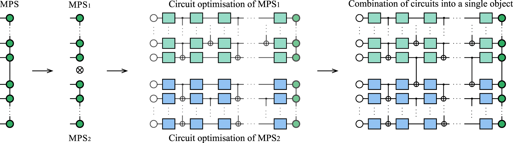
If a single cut is not enough, we cut each MPS again into halves and apply this algorithm recursively.
In the numerical experiments, we have found that a single run of this procedure is sufficient to optimize the 100-qubit circuit with 3 layers for the preparation of the Gaussian density function  on the interval
 ![$[0,1]$](https://content.cld.iop.org/journals/2058-9565/8/3/035027/revision2/qstacd9e7ieqn85.gif) with a
with a  approximation fidelity. At the same time, the state preparation algorithm implemented on the full 100-qubit circuit without any cuts prepares the same state with the fidelity close to zero.
4. Conclusion
We have extended the fruitful idea of MPS-based encoding schemes by considering variational hardware-efficient circuits as an encoder for high-dimensional vectors. The derived protocol allows us to solve the problem of efficient encoding of structured classical data into a multi-qubit quantum state. Examples of such data are smooth functions [45], probability distributions [55], videos [56], and image classifiers [57, 58].
As an illustrative example, we consider the preparation of states generated by specific analytical functions utilizing variational circuits with the canonical quantum gate set and restricting the connectivity to neighbor qubits. The latter assumption benefits not only physical realization, but also tensor-based simulations [47, 54], which we exploit to optimize the circuit parameters. We show that shallow circuits suffice to approximate considered functions with a high accuracy.
Our method can be applied to a wide variety of quantum algorithms. Firstly, partial differential equations (PDEs) after discretization are reduced to a system of linear equations Ax = b, where b is usually obtained by sampling an analytical function on an interval. All quantum linear system solvers [1–5] require preparation of b as the first step. Secondly, preparation of probability distribution functions is the main subroutine in calculation of the expectation values, which is a central problem in the finance [7, 12], e.g. risk analysis [6], and option pricing [59]. In addition, preparation of distributions can be applied to the sampling tasks [53, 60, 61]in computational statistics and quantum mechanics. One of the main bottlenecks in quantum machine learning [8, 62, 63] is the absence of quantum random access memory [64]. Our approach can be applied to the encoding of structured data, such as images [41, 65] and videos [56], into quantum circuits. Besides, our method can be utilized to prepare quantum states for sensing to maximise the detection efficiency [66, 67]. A more detailed explanation of these applications is given in appendix
It is worth mentioning that  points are sufficient for the discretization of a single-variable function in the majority of problems, which requires 20–30 qubits. Higher number of qubits is necessary for multi-parameter functions, where our approach works as well in case when the correlations between variables are relatively small. Such multi-parameters functions are arising in the multi-dimensional PDEs [68], option pricing [69] and other problems [70]. The preparation of high-dimensional vectors requires large quantum circuits, which are generally hard to optimize due to the barren plateaus. Here we proposed a 'cut once, measure twice' approach that facilities the circuit optimization by proper initialization.
We also investigated circuits of different structures and found that there is no superior architecture, leaving the choice of the circuit to the user or hardware topology. Our algorithm is generic and can be applied to an arbitrary circuit, where variational gates may be applied over multiple qubits and/or defined by the hardware, e.g. rf-pulses, laser radiation, etc.
Following the paradigm of hybrid classical–quantum computing, we expect tensor-based algorithms to be the method of choice since the classical tensor networks subroutines feature logarithmic complexity in memory consumption and runtime and can be easily translated to quantum hardware for further manipulations. Mainly, the classical part can be done via tensor networks and then its output is transferred to a quantum computer with the help of our algorithm. Besides, the output quantum state vector that is well described as an MPS can be obtained using logarithmic—in the vector size—number of measurements [71]. Such an approach concludes the full cycle of hybrid computation MPS  QC
QC  MPS, where all steps performed in logarithmic complexity.
Acknowledgments
The work of Ar A M, A A T, F N, and M R P was supported by Terra Quantum A G. The work of S V D was financially supported by Terra Quantum A G through the consultancy agreement.
Ar A M, A A T and M R P devised the algorithm. A A T wrote the code and performed the experiments. Ar A M, S V D, M R P, A A T analyzed and improved the algorithm. F N and M R P supervised the project. All authors discussed the results, wrote the manuscript and contributed to the work.
Data availability statement
No new data were created or analysed in this study.
Appendix A: Software
We perform quantum circuits simulation using the QMware system [72]. The circuits are assembled using QASM language and are, therefore, library-agnostic, i.e. can be run using Cirq, Qiskit, PennyLane, etc. We implement the proposed algorithm as Python library QPrep, which is publicly available in [73]. The library requires a function, number of sampling points and layers as an input and provides a circuit for the corresponding quantum state preparation.
Appendix B: Riemannian optimization
Riemannian optimization allows us to optimize a function constrained on a Riemannian manifold. In this work, our purpose is to minimize the infidelity equation (2) on the manifold of isometric matrices. We calculate the (Euclidean) gradient, find its projection onto the tangent space, and project the updated matrix onto the space of isometric matrices.
Here, we denote the manifold of isometric matrices of size  as
as  and the tangent space at point
  as
as  . The Riemannian gradient of some differentiable function f(X) at point
  of isometric matrices is calculated as (see supplemental material, section 4 for further details)

By definition,  is an orthogonal projection of the Euclidean gradient
  onto the tangent space
  . The last step is the projection of the updated matrix
  on the manifold of isometric matrices
  , which is performed via SVD-retraction:

where  is the SVD decomposition.
Appendix C: Applications
C.1. Sampling
The most straightforward way to apply quantum state preparation is the sampling task [31]. Our algorithm allows for the preparation of probability distribution functions, and then measurement of qubit's states provides us samples. For instance, the function of interest can be the Gaussian distribution, that has restricted MPS ranks in case of good structure of the covariance matrix (small ranks of off-diagonal blocks of the matrix) [74].
C.2. Solution of linear systems of equations
Linear systems of equations usually arise considering partial differential equations after their discretization. For instance, simple one-dimensional Poisson equation

gives the system of linear equations that can be discretized on the uniform grid

where  is the function value at the corresponding point.
Most of quantum algorithms for linear systems assumes that it is possible to efficiently prepare any desired state b [1, 3, 5]. However, there is still no general and established framework for this task and we expect that our approach facilitates the vectors encoding.
C.3. Expectation value calculation
Calculation of the expectation value is one of the main routine in the computational finance, and many quantum algorithms are devoted to this problem [7, 12]. At the same time, the quantum state preparation is one of the main subroutine in these approaches, so our method is applied here as well.
For example, in the risk analysis, the Value at Risk needs to be calculated [6]. That is to find the smallest X such that:

for fixed α. This can be reformulated to calculation of the expectation value of the Heaviside step function  with various values of X. Suppose we have distribution function p(x) defined on the interval (a, b), then:

Thus, the task is reduced to finding the expectation value. If one wants to calculate it on a quantum computer one can use the amplitude estimation algorithm [75] which provides quadratically better error scaling than classical Monte Carlo. But first of all, one needs to prepare the distribution function p(x) discretized on the interval (a, b):

Supplementary data (0.2 MB PDF)