

Abstract
Monitoring national and global greenhouse gas (GHG) emissions is a critical component of the Paris Agreement, necessary to verify collective activities to reduce GHG emissions. Top-down approaches to infer GHG emission estimates from atmospheric data are widely recognized as a useful tool to independently verify emission inventories reported by individual countries under the United Nation Framework Convention on Climate Change. Conventional top-down atmospheric inversion methods often prescribe fossil fuel CO2 emissions (FFCO2) and fit the resulting model values to atmospheric CO2 observations by adjusting natural terrestrial and ocean flux estimates. This approach implicitly assumes that we have perfect knowledge of FFCO2 and that any gap in our understanding of atmospheric CO2 data can be explained by natural fluxes; consequently, it also limits our ability to quantify non-FFCO2 emissions. Using two independent FFCO2 emission inventories, we show that differences in sub-annual emission distributions are aliased to the corresponding posterior natural flux estimates. Over China, for example, where the two inventories show significantly different seasonal variations in FFCO2, the resulting differences in national-scale flux estimates are small but are significant on the subnational scale. We compare natural CO2 flux estimates inferred from in-situ and satellite observations. We find that sparsely distributed in-situ observations are best suited for quantifying natural fluxes and large-scale carbon budgets and less suitable for quantifying FFCO2 errors. Satellite data provide us with the best opportunity to quantify FFCO2 emission errors; a similar result is achievable using dense, regional in-situ measurement networks. Enhancing the top-down flux estimation capability for inventory verification requires a coordinated activity to (a) improve GHG inventories; (b) extend methods that take full advantage of measurements of trace gases that are co-emitted during combustion; and (c) improve atmospheric transport models.
Export citation and abstract BibTeX RIS

Original content from this work may be used under the terms of the Creative Commons Attribution 4.0 license. Any further distribution of this work must maintain attribution to the author(s) and the title of the work, journal citation and DOI.
1. Introduction
Success of the Paris Agreement (UNFCCC 2023a) relies on accurately monitoring and verifying collective global greenhouse gas (GHG) emissions reduction efforts. We cannot afford not to have these systemic checks and balances if we are to minimize further global mean surface warming of Earth. Following preceding environmental protocols, such as the Kyoto protocol (UNFCCC 2023b), national emission inventories (NEIs) will play a key in role in planning and reporting reductions in GHG emissions. The emission reporting is a minimal regulatory obligation under the Paris Agreement by all submitting parties, including countries who had not reported a NEI under the previous Kyoto Protocol, unlike developed nations called Annex I countries. Robustness of inventory estimates requires a clear, transparent, and consistent framework for data collection, analysis, and compilation. In addition to the inventory capacity building for the new inventory submissions, the enhanced evaluation and verification of reported inventory estimates (e.g. IPCC 2019) should further reinforce the global emission reduction monitoring and assure the global compliance of pledged climate mitigation efforts (e.g. nationally determined contribution (NDC)); however, due to the nature of the activity-data based emission calculation (e.g. IPCC 2006), where emissions are assumed to be proportional to activity levels, even with an established framework, inventory emission estimates are intrinsically prone to systematic biases due to emission factors and activity data used (e.g. Guan et al 2012, Liu et al 2015). Assuring the accuracy of NEI emission estimates is critical in the technical assessment of our climate mitigation progress towards the temperature goal (Weir et al 2022).
The use of atmospheric data for evaluating and verifying GHG emissions has been extensively examined over the past decades (e.g. NRC 2010, NAMES 2022). Generally, changes in the atmospheric concentration of trace gases are due to emissions, uptake, and atmospheric chemistry and transport. In the case of atmospheric CO2, changes are largely determined by fluxes (emissions minus uptake) and atmospheric transport (e.g. Palmer et al 2008). Atmospheric CO2 flux inversions take advantage of the information provided by atmospheric data to CO2 flux estimates (e.g. Tans et al 1990, Gurney et al 2002). While flux inversions started as an approach to estimate the size and location of large-scale sources and sinks (e.g. Tans et al 1990, Gurney et al 2002), the methods are now widely recognized as a potential tool for the QA/QC and verification of NEIs (e.g. IPCC 2019). Atmospheric top-down approaches also provide an opportunity for determining national emission estimates from countries that do not currently have the infrastructure to robustly provide bottom-up emission estimates. NEIs provide annual country level emissions, while the Paris Agreement recognizes the subnational key actors as the driving force for the progress. Atmospheric top-down approaches should be also able to fill the information gaps and provide actionable estimates for key sub-national targets, such as states, provinces, cities, subject to data coverage.
Top-down flux estimation methods rely on prior emission estimates and meteorological reanlayses to drive the atmospheric transport model to determine 3D atmospheric concentrations of CO2 that are subsequently sampled subject to the instrument sampling configurations. Most inverse methods use Bayes' theorem to fit optimal distributions of CO2 fluxes that minimize the mismatch between model and observations of CO2, subject to model and measurements uncertainties. The resulting posteriornet fluxes of CO2 are consistent with prior knowledge and measurements, and their uncertainties. A common approach adopted by top-down flux estimation methods is then to subtract the prior fossil fuel emissions from the posterior net flux estimates to quantify natural fluxes (e.g. Gurney et al 2005, Wang et al 2020, Byrne et al 2023). First, this implicitly assumes perfect knowledge of fossil fuel CO2 emissions (FFCO2, roughly corresponding to emissions from energy sector). Consequently, the prior model and observation mismatch (and the associated uncertainties) is attributed exclusively to incorrect natural biosphere fluxes. FFCO2 is not corrected in this process so errors in the magnitude of FFCO2 will be redistributed to the posterior flux estimate for the natural biosphere. This limits the current use of top-down estimates for evaluating country emissions only to the portion of CO2 emission that excludes energy sector CO2, i.e. agriculture, forestry and land use. Second, any assumption about the spatial and temporal variations in FFCO2 will leave a residual in the posterior solution, irrespective of the subtraction of the prior (e.g. Oda et al 2019, Wang et al 2020). It is important to note that top-down methods also suffer from their own errors, and there are still large discrepancies in posterior regional fluxes estimated by using different approaches (e.g. Peylin et al 2013, Houweling et al 2015, Takagi et al 2015, Crowell et al 2019), partially due to differences in atmospheric transport modeling (e.g. Schuh et al 2019).
In this study, we investigate how different assumptions about FFCO2 inventories, particularly temporal changes, can imprint themselves onto posterior flux estimates. For this work we use the independent ODIAC and GridFED emission inventories, which were used in the recent inversion-based inventory assessment prototyping studies, such as Deng et al (2022) and Byrne et al (2022), to help drive the GEOS-Chem model of atmospheric CO2. We use the inventory difference as an estimate of FFCO2 errors. An established ensemble Kalman Filter (EnKF) is used to infer posterior net CO2 fluxes from in-situ and satellite data. We describe the GEOS-Chem and its CO2 inventories, the EnKF, and the in-situ and satellite data in next section. In section 3, we report our results and explore how differences the two FFCO2 emission inventories play a role in posterior fluxes estimates for the natural biosphere. We conclude the paper in section 4 with a broader discussion of our results and recommendations for further work.
2. Methods
2.1. Fossil fuel CO2 emission datasets
We used two different FFCO2 gridded data products used in large international projects: ODIAC and GridFED. The summary of two gridded emissions is shown in table 1. These gridded emission products are both based on the downscaling of country-level emissions. The differences between the two emission products are largely attributable to the underlying emission estimates and the spatial and temporal downscaling methods used.
Table 1. A summary of two FFCO2 gridded emission data products used in this study.
| Emission estimates | Spatial patterns | Seasonality | Reference | |
|---|---|---|---|---|
| ODIAC2019 | CDIAC reference approach using United Nations Statistics Division (UNSD) data | Downscaling using point sources and Nighttime lights | Based on monthly fuel consumption from top-emitting countries (see Andres et al 2011) | Oda et al (2018) |
| GCP-GridFED (2019) | UNFCCC reported sectoral emissions for Annex I countries; CDIAC estimates for the rest of the world | Adopted EDGAR v4.3.2 sectorally downscaled maps | Defined by geographical zone and sector using proxy data (see Janssens-Maenhout et al 2019) | Jones et al (2021) |
ODIAC is a global high-resolution FFCO2 data product (Oda and Maksyutov 2011, Oda et al 2018). ODIAC distributes global and country level emission estimates made by the Carbon Dioxide Information and Analysis Center (CDIAC) at the Appalachian State University (CDIAC at AppState, hereafter CDIAC, Gilfillan et al 2021). CDIAC estimates are based on energy data (e.g. fuel production and consumption) collected by the United Nation Statistical Division. CDIAC country estimates are based on the fuel consumption using the approach developed by Marland and Rotty (1984), so called reference approach (e.g. IPCC 2006), are reported by fuel type (oil, gas, and coal). The reference approach is also used for evaluation of the reported emissions using the sectoral approach where emissions are reported for key emission sectors (e.g. IPCC 2006). Historically, CDIAC also reports emissions from cement production and gas flaring as part of FFCO2 (e.g. Marland and Rotty 1984, Andres et al 2012). ODIAC distributes the country emissions using point source information and satellite-observed nightlight data to a global 1 km domain (e.g. Oda and Maksyutov 2011). The emission seasonality in ODIAC is based on the analysis of Andres et al (2011). The Andres 2011 seasonality is based on the top 20 emitting countries' fuel consumption data. ODIAC has been used in a number of atmospheric CO2 simulations and flux inversion studies at different scales, such as global (e.g. Maksyutov et al 2013, 2021, Crowell et al 2019, Palmer et al 2019, Liu et al 2021, Wang et al 2020), regional (e.g. Fischer et al 2017, Feng et al 2019) and local/city scales (e.g. Lauvaux et al 2016, 2020, Oda et al 2017, Hedelius et al 2018, Roten et al 2022), including the recent model intercomparison activity under NASA's Orbiting Carbon Observatory (OCO) mission (Byrne et al 2023).
GCP-GridFED relies on the well-established EDGAR emission database. GCP-GridFED also uses CDIAC country emissions, but only for non-Annex I countries, who have not regularly submitted NEIs every year. Emission estimates for Annex I countries are taken from NEIs reported to United Nation Framework Convention on Climate Change (UNFCCC). NEIs are often compiled following the established IPCC guidelines (e.g. IPCC 2006). Emissions are calculated and reported by key emission sector using the sectoral approach (e.g. IPCC 2006). The reference approach, which CDIAC is based on, should agree with the sectoral approach-based emissions for energy sector (IPCC 2006), with small differences due to non-energy use (e.g. Marland and Rotty 1984) and thus is used for checked the calculate totals. The IPCC guidelines recommend better emission factors (EF) if available other than ones provided by the default values provided by the IPCC EF database. The activity data (e.g. fuel consumption) are not necessarily identical with ones reported to UNSD. Due to these differences, the GCP-GridFED total does not fully agree with the original CDIAC total (and, consequently, ODIAC). The sectoral country total emissions are mapped at approximately 10 km resolution using the EDGAR v4.3.2 sectoral maps developed for the year 2010 (Janssens-Maenhout et al 2019). The emission seasonality in GCP-GridFED is based on the analysis by Janssens-Maenhout et al (2019), which is based on the geographical region-based proxy approach. Further details can be found elsewhere (Jones et al 2021).
In this study, we used the differences of two products as an estimate of potential errors and uncertainties in FFCO2. The comparison of the two products for the winter and summer in 2017 is presented in figure S1. We solely focus on the impact of the different emission seasonality for the following reasons. First, the country level FFCO2 emissions are often very similar regardless of the methodologies (e.g. Andres et al 2012). Second, it is reasonable to assume the spatial differences (downscaling errors) are significantly mitigated when the emission products are mapped onto a coarse spatial resolution model domain (2 x 2.5 degree in this study, see 2.2). It has been previously demonstrated that spatial aggregation should mitigate the downscaling errors (e.g. Oda et al 2019). A previous study also examined the impact of the emission downscaling errors on the inverse estimates (Wang et al 2020). The evaluation of the downscaling error has been done in several previous studies (e.g. Oda et al 2018, 2019). Both ODIAC and EDGAR gridded emissions were extensively evaluated, and the potential errors were characterized over China at multiple key policy relevant scales (Han et al 2020a, 2020b, 2020c). It is important to note that the emission seasonality should have a direct impact on the simulated results and the subsequent analysis in combination of other temporally varying meteorology and surface fluxes. Unlike the spatial downscaling errors, the impact cannot be mitigated.
2.2. Flux inversion system
We use an EnKF framework (Feng et al 2017, Palmer et al 2019) to estimate surface CO2 fluxes from atmospheric CO2 data collected by a satellite and a global in-situ ground-based observation network during 4 years from 2015 to 2018, inclusively. We define our land sub-regions by dividing each of the 11 TransCom-3 land regions (Gurney et al 2002) into 30 nearly equal sub-regions, with the exception for temperate Eurasia that has been divided into 56 sub-regions, due to its large landmass. We further divide 11 TransCom-3 oceanic regions into 132 sub-regions. Our state vector includes monthly scaling factors for 488 regional pulse-like basis functions that describe natural CO2 fluxes, including 356 land regions and 132 oceanic regions (see figure S2). The inversion experiments closely follow Palmer et al (2019) in which they assimilate in-situ data and column averaged CO2 dry-air mole fraction (XCO2) retrievals of version 10 r from the NASA OCO-2 satellite that was launched in 2014. To reduce possible model transport and representation errors, we run the (GEOS-Chem) global transport simulation at a spatial resolution of 2° × 2.5°.
The simulations are forced by predefined a priori CO2 flux inventories, which include natural fluxes of: (1) monthly biomass burning emission (GFEDv4.1; van der Werf et al 2010); (2) monthly climatological ocean fluxes (Takahashi et al 2009); and (3) 3-hourly terrestrial biosphere fluxes (CASA; Olsen and Randerson 2004), and (4) the anthropogenic emissions, prescribed by two different FFCO2 product of (a) ODIAC v2020 (referred as ODIAC); or (b) GridFED (referred as GCP thereafter). As a result, any difference in the resulting posterior fluxes (and model concentrations) can be fully attributed to difference in FFCO2.
2.3. Observational data
We use the OCO-2 XCO2 retrievals of version v10r by the JPL-ACOS team (Taylor et al 2023). We only assimilate the nadir and glint observations over land, considering possible bias between the land and ocean XCO2 data (Peiro et al 2022). Also, to reduce the computational costs and error correlations, we thinned the observation time series to ensure a minimal time interval of 10 s. In companion sensitivity experiments, we assimilated data from (a subset of) 113 sites (figure S2 in appendix) included in the NOAA data collection of the GLOBALVIEWPlus 7.0 for atmospheric CO2 observations by the global in-situ network (see Schuldt et al 2021 for more details).
3. Results
3.1. FFCO2 uncertainty challenge in flux inversions
Figure 1 shows the prior and the posterior net fluxes (fossil + land biosphere + fires + oceans) from two satellite data inversions that use different FFCO2 products (section 2.1). Results are shown for global, over aggregated continental regions (northern land and tropical land) and large source areas/countries (North America, China and Europe). We primarily focus on the land fluxes because FFCO2 plays only a small role in the size of ocean fluxes. At these large spatial scales, the differences between two sets of inversions, including prior and posterior fluxes, are small compared to the magnitude of the net prior and posterior fluxes. The difference plots of two inversions (smaller panels in figure 1) show that the seasonal amplitude of the global flux difference is ∼0.15 PgC/month, corresponding to ∼4% of the global CO2 flux seasonal amplitude (∼3.5 PgC/month). These differences in the global fluxes are largely attributable to the emissions from the Northern Hemisphere where most of the large emitting countries, including the top emitting countries, such as China, the U.S, and India (based on Gilfillan and Marland 2021), are located (see global and North Land plots).

Figure 1. Prior and posterior net fluxes (fossil + land biosphere + fires + oceans) from two satellite data inversions with ODIAC and GCP-GridFED and the differences. Shown for global and over aggregated large regions, such as northern land, tropical land, North America, China, and Europe. Both sets of prior (black and green dash) and posterior (red and blue) from two inversion cases are almost identical in this presentation and overlapped (green dash under back, and red under blue).
Download figure:
Standard image High-resolution imageThese difference plots in figure 1 also illustrate the challenge of correctly prescribing a seasonal component of FFCO2. Differences introduced by competing assumptions about seasonal FFCO2 in the prior fluxes are largely eliminated in the posterior fluxes via flux optimization inversion. The posterior fluxes associated with using ODIAC are slightly larger than those that use GridFED. We find that the substantially reduced seasonal difference in net posterior fluxes is due to a compensating seasonal cycle for posterior natural fluxes (terrestrial biosphere and oceans). In short, the inversion has successfully fitted net CO2 fluxes (the sum of fixed FFCO2 and adjusted natural fluxes) to atmospheric CO2 concentrations by adjusting only the natural fluxes, which will potentially also include an adjustment due to an erroneous seasonal cycle for FFCO2. This misattribution of the FFCO2 seasonality to the natural fluxes is common to all the inversions we present. This misattribution error is more problematic for countries that are not spatially well-resolved by the available data the resolution of flux estimations, with the impact proportional to the magnitude of emissions, as discussed earlier. For example, 75% of the countries and territories in the world are smaller than the typical size of the land sub region in the inversion system (approximately, 500 000 km2) (https://en.wikipedia.org/wiki/List_of_countries_and_dependencies_by_area). Accurately prescribing sub-annual FFCO2 is therefore crucial to obtain robust flux estimates, especially for obtaining continental country specific emission estimates in support of inventory evaluation.
3.2. How are FFCO2 seasonal differences imprinted on net and land biosphere fluxes?
The misattribution error described above is exacerbated especially when prior FFCO2 is then subtracted from the posterior net fluxes to estimate the posterior natural fluxes, a typical approach that implicitly assumes that FFCO2 errors are much smaller than natural flux errors. Figure 2 shows the posterior natural flux maps and the difference map for boreal summer (June, July and August) and winter (December, January and February) months for both sets of inversions that use satellite and in-situ data. All the inversions use the same prior natural flux inventories, and differences in their prior FFCO2 inventories are shown in figure S1. The large spatial patterns of posterior net fluxes are similar among the cases (see panels of the top two rows in figure 2), as expected. We focus on the differences between inversions that use different FFCO2, which show the influence of assuming different FFCO2 seasonality on the posterior natural flux estimates. Noticeable differences are over the major emitting areas, including China, the U.S, and Europe, consistent with the continental-scale net fluxes (figure 1). We find that the influences of FFCO2 differences on natural fluxes are significant (∼40% of the natural portion of the net fluxes, see figure S3) on sub-continental scales.
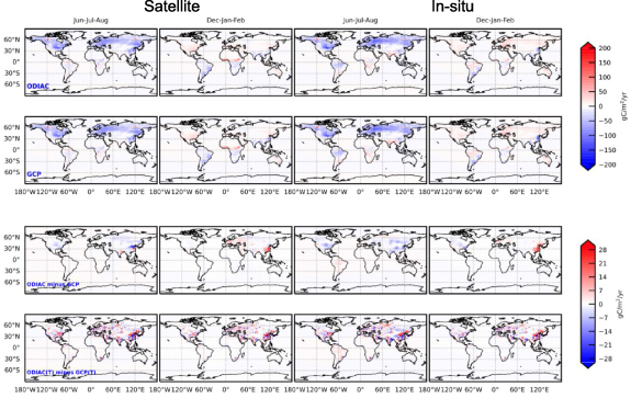
Figure 2. Posterior natural fluxes from satellite inversions (left two columns) and in-situ inversions (right two columns). The top two rows show results posterior flux using ODIAC and GCP-GridFED. The bottom two rows show difference in estimated natural and net (including FFCO2) fluxes.
Download figure:
Standard image High-resolution imageComparing posterior natural fluxes inferred from satellite data (left two columns in figure 2) and in-situ data (right two columns in figure 2), we find that posterior differences are larger for the inversion that uses satellite data than the inversion that uses in-situ data over the regions where FFCO2 discrepancies are largest. This is largely because the ground-based network sites are historically (and intentionally) placed at remote geographical locations, where fossil fuel contributions are minor, to support background monitoring of atmospheric CO2 and other gases. Thus, the posterior fluxes from in-situ inversions should be less sensitive to FFCO2 errors compared to the inversion case with satellite data because of the spatial coverage and/or density differences between two observation systems. Conversely, the in-situ inversion tends to mitigate more of the difference in FFCO2 inventories over remote areas which are poorly constrained by observations, such as central and west China. Generally, we find that satellite observations provide denser spatial coverage compared to the ground network, acknowledging that satellite data represent different information to the in-situ data, i.e. column averaged CO2 retrieved from radiance measurements compared to CO2 mole fractions sampled in the lower troposphere. Obtaining robust flux estimates with improved spatial resolutions requires dense CO2 data. Satellites, such as NASA's OCO-2 and Japan's GOSAT, have collected data globally, including geographical gaps left by the ground-based global reference network.
The smaller posterior flux differences due to different assumptions about seasonal changes in FFCO2 when we use satellite data, compared to when we use in-situ data, are seemingly a welcome result. However, they also highlight the challenge of dealing with FFCO2 contributions, especially in the satellite flux inversion framework, because of the sensitivity of the observations to FFCO2. It is important to reiterate that we find that the inversion system adjusted the natural fluxes to help compensate for FFCO2 differences. It is also important to note that the flux differences between the inversions that use different FFCO2 products are still smaller than the difference between inversions that use satellite and in-situ data (see figure S4).
Figure 3 shows the posterior model CO2 concentration differences, inferred from OCO-2 XCO2 retrievals, resulting from using the different FFCO2 inventories. We present differences for the boundary layer and total dry-air column XCO2 for both the winter (January, 2017) and summer (July, 2017) cases, to show the FFCO2 error sensitivity for the future space-borne and surface-based observation systems, in addition to using the current OCO-2 constraints. As expected, the impact of the FFCO2 errors are more significant near the surface and near the source regions. Some of the FFCO2 errors were not corrected even after the model had been fitted to the data (see figure S5). For example, the posterior concentration fields show 0.5 ppm differences in the boundary layer over the high northern latitudes. Historically, ground-based observations are often located far from those intense emission areas, but recent (and planned future) dense regional networks, such as Europe (Heiskanen et al 2022), North America (e.g. Karion et al 2020), and East China, can detect those differences (of up to 4 ppm) and therefore represent potentially useful constraints on local FFCO2 inventories. In contrast, XCO2 differences are more spread out and planned satellites missions (of which the most prominent example is the upcoming Copernicus CO2 Monitoring mission, CO2M) should be able to pick up these differences and minimize the misattribution of errors in prior inventories between regions with different observation constraints. This suggests that satellite-based inversions are in a better position going forward to serve as a global tool for the QA/QC and verification due to its global dense observation coverage. Typically, the differences showed below are within the model errors assigned (for example, 1–2 ppm, Schuh et al 2019). The increased observation coverage might lead to a need for reassessing the model-observation mismatch values based on the FFCO2 differences. As seen in the flux map comparison, we find the largest differences over high-emitting areas, such as US coastal, Europe and China/India, while the differences are more confined locally in the case of boundary layer and XCO2 differences are less pronounced and less localized over geographical region where in-situ data are particularly sparse.

Figure 3. FFCO2 differences (ODIAC minus GCP) seen in the prior concentration fields (top: Boundary layer; Bottom: XCO2) for winter (January) and summer (July).
Download figure:
Standard image High-resolution image
4. Discussion
Under the Paris Agreement, new mechanisms, such as submission of NDC and the Global Stocktake (GST), are introduced to achieve the temperature goal via our global collective efforts. In addition to mandatory emission reporting to UNFCCC, each signatory country must submit a NDC that describes their GHG emission reduction goals, trajectory, and the approaches they will use to achieve that trajectory. GST is an evaluation process of our progress towards the Paris Agreement goal. GST is planned to be held every five years and the results of the assessment are used to set more stringent target in the next NDCs. Currently the very first GST is underway. In addition to the synthesis reports, such as IPCC reports, GST is the technical assessment process where science-based approaches should be fully utilized to address the guiding mitigation and adaptation questions.
While the NEIs submitted to UNFCCC remain the fundamental tool to keep track of emission changes of parties, the use of NEIs for fully addressing the mitigation guiding questions in GST is challenging. For example, NEIs might not cover all the sources and sinks that we need for global assessment using earth system models, but emissions from the key sectors for individual countries. The NEIs are specifically designed to keep track of emission changes from the countries. Depending on the data and capacity availability, estimates could be obtained with different levels of details (Tier 1–3) and thus emissions from different countries might not be comparable due to the underlying data and emission factors. While NEIs should cover key GHG emission sectors for countries, the emission might not be complete to represent all the GHG emissions from the domain for the year of interest. NEIs also do not cover emissions from international marine bunkers and aviation. Moreover, as discussed earlier, the emissions are not provided beyond country and annual scales. Thus, the global emission products have a key role in the technical assessment in GST to supplement the emission information that we cannot obtain solely from NEIs.
The use of gridded emissions allows us to perform atmospheric data-based emission analyses, such as atmospheric inversions. Several studies have reported anthropogenic emission estimates determined by inversion approaches, but these are often limited to relatively small spatial scales, such as cities and local sources (e.g. Lauvaux et al 2020). Large scale inversions, which typically estimate fluxes on spatial scales comparable to NEIs, are often done in a conservative way that avoid the direct estimation of FFCO2, with some exceptions, e.g. Maksyutov et al (2021). Consequently, the current focus of CO2 inventory evaluation using inversions has been the Agriculture, Forestry and Other Land Use sector (e.g. Deng et al 2022, Byrne et al 2022). Our results demonstrated that inversions compensate the FFCO2 errors, but the corresponding flux corrections are attributed exclusively to the natural fluxes. To effectively evaluate NEIs using atmospheric inversions, we would need improvements to the current inversion approaches. Flux resolutions of inversions might be often too large to resolve individual countries, especially for small countries. Previous studies have examined the missing sources in many inversions, such as CO2 from oxidation of reduced carbon species (e.g. Wang et al 2020).
To improve the ability of estimating anthropogenic emissions and other combustion emissions, such as fires, the use of multiple species should be also considered. Ultimately, this is a necessary step because reporting net fluxes of CO2 are not enough to describe the collective assessment in a GST, especially addressing the guiding questions. Effective mitigation of national emissions of anthropogenic GHGs requires reliable knowledge of emissions from individual contributing sectors. Sector emissions of CO2 are typically accompanied by a range of trace gases that are typically measured by the air quality (AQ) community, some of which are also observed by Earth-observing satellites, e.g. carbon monoxide and nitrogen dioxide that are used commonly as tracers for incomplete combustion. A synergy of GHG and AQ measurements is there important to support the mitigation of GHG emissions, including at least better coordination of GHG and AQ measurement networks. The U.S. and Europe have extensive ground-based observation networks (e.g. NOAA and ICOS) and some of the sites have been used to study FFCO2 (e.g. Basu et al 2020). We also need to improve modeling of atmospheric transport (Simmonds et al 2021) and chemistry to help reduce the uncertainties associated atmospheric transport that are often the dominant error component in inversions (e.g. Schuh et al 2019).
Ideally, GHG inventories should be developed in a way to fully utilize the model and observations. Given the timeline of UNFCCC framework, the efforts made by the scientific inventory community will help fill the knowledge gaps and guide the framework to be more responsive to the evolving needs of climate mitigation. We argue that an extended data collection would greatly help improving the utility of inversions. For example, the use of the subnational data as noted by IPCC (2019) is optional, but it is an effective way to improve the description of emissions in space and time. As we showed in our study, obtaining robust seasonal emission estimates should directly improve the accuracy of inversion results especially reducing the impact of large emitting countries. The availability of the activity data for emission calculation at subnational scales, especially cities, could be limited and the robustness of the system boundary calculation is lower in theory.
Temporal emission disaggregation is challenging due to the limited data availability. Andres et al (2011) was based on the fuel data collected from the top 20 emission countries. The uncertainty associated with the temporal component was about 15%–20%. Beyond monthly scales, there are not many options for us to implement downscaling (e.g. Nassar et al 2013, Crippa et al 2020). The use of alternative activity data has emerged (e.g. Le Quéré et al 2020, Liu et al 2020), but the accuracy of the resulting emissions are not fully evaluated. The expected uncertainty should be much higher than what we typical expected from inventory estimates based on fuel consumption (Oda et al 2021). The incremental approach is suitable for near-real time (NRT), but it does not provide total constrain and thus could be biased (see figure S6). For example, most of the emissions in NRT CO2 emissions were represented by US and China data where emission calculations were well supported by statistical data. For these reasons, an established framework could take a role as clearing house to coordinate data collection for NEIs and GST. Looking ahead, capacity building for the development of reliable inventories in the projected large emitting countries is important.
5. Conclusions
We examined the impact of the FFCO2 errors on the flux inversion results using two observation systems. We revisited the FFCO2 assumption, one of the obstacles in the conventional flux inversion for serving as a tool for QA/QC and evaluation/variation of reported NEIs as well as potentially providing GHG estimates for countries with less robust inventory capacity and examined the impact of the inverse estimates using two inventories that approximate FFCO2 errors. We demonstrated how FFCO2 errors can cause biases in posterior flux estimates. The magnitude of the errors are small compared to the magnitude of natural fluxes and on national scales but can be significant on subnational scales. We found that differences in the prior seasonal differences in FFCO2 are the largest driver for the estimation of natural fluxes. We found that errors associated with prescribing seasonal emissions are larger and more direct than errors associated with prescribing the spatial distribution of emissions. For the use of inversions for inventory evaluation, we need robust sub-annual estimates for FFCO2, especially for large emitting countries such as China, to quantify robust top-down emission estimates, particularly at policy-relevant national and subnational scales. Extended data collection would directly improve accuracy of inverse estimates for science and global monitoring of GHG emissions under the Paris Agreement.
We found that satellite data provide us with the best opportunity to quantify FFCO2 emission errors; a similar result is achievable using dense, regional in-situ measurement networks. Therefore, they provide a better option to evaluate national emission inventories. However, the corresponding top-down flux corrections associated with errors in FFCO2 are attributed to natural flux estimates by virtue of a common approach adopted by inverse methods, which implicitly assumes that we have perfect knowledge of FFCO2. To help improve the evaluation of NEIs and the technical assessment in the GST, inversions need to improve the accuracy of their estimates and to improve knowledge of the processes that explain the difference between models and atmospheric data, e.g. emissions, atmospheric transport.
Acknowledgments
T O is supported by NASA Grant # 80NSSC21K1929. L F and P I P acknowledge support from the UK National Centre for Earth Observation funded by the Natural Environment Research Council (NE/R016518/1). Authors acknowledge contribution of the following invividuals to the ObsPack CO2 GLOBALVIEWplus product (v7.0): Kenneth N Schuldt, John Mund, Ingrid T Luijkx, Tuula Aalto, James B Abshire, Ken Aikin, Arlyn Andrews, Shuji Aoki, Francesco Apadula, Bianca Baier, Peter Bakwin, Jakub Bartyzel, Gilles Bentz, Peter Bergamaschi, Andreas Beyersdorf, Tobias Biermann, Sebastien C Biraud, Harald Boenisch, David Bowling, Gordon Brailsford, Gao Chen, Huilin Chen, Lukasz Chmura, Shane Clark, Sites Climadat, Aurelie Colomb, Roisin Commane, Sébastien Conil, Adam Cox, Paolo Cristofanelli, Emilio Cuevas, Roger Curcoll, Bruce Daube, Kenneth Davis, Martine De Mazière, Stephan De Wekker, Julian Della Coletta, Marc Delmotte, Joshua P DiGangi, Ed Dlugokencky, James W Elkins, Lukas Emmenegger, Shuangxi Fang, Marc L Fischer, Grant Forster, Arnoud Frumau, Michal Galkowski, Luciana V Gatti, Torsten Gehrlein, Christoph Gerbig, Francois Gheusi, Emanuel Gloor, Vanessa Gomez-Trueba, Daisuke Goto, Tim Griffis, Samuel Hammer, Chad Hanson, László Haszpra, Juha Hatakka, Martin Heimann, Michal Heliasz, Arjan Hensen, Ove Hermanssen, Eric Hintsa, Jutta Holst, Viktor Ivakhov, Dan Jaffe, Warren Joubert, Anna Karion, Stephan R Kawa, Victor Kazan, Ralph Keeling, Petri Keronen, Pasi Kolari, Katerina Kominkova, Eric Kort, Elena Kozlova, Paul Krummel, Dagmar Kubistin, Casper Labuschagne, David H Lam, Ray Langenfelds, Olivier Laurent, Tuomas Laurila, Thomas Lauvaux, Jost Lavric, Bev Law, Olivia S Lee, John Lee, Irene Lehner, Reimo Leppert, Markus Leuenberger, Ingeborg Levin, Janne Levula, John Lin, Matthias Lindauer, Zoe Loh, Morgan Lopez, Toshinobu Machida, Ivan Mammarella, Giovanni Manca, Andrew Manning, Alistair Manning, Michal V Marek, Melissa Y Martin, Hidekazu Matsueda, Kathryn McKain, Harro Meijer, Frank Meinhardt, Lynne Merchant, N Mihalopoulos, Natasha Miles, Charles E Miller, John B Miller, Logan Mitchell, Stephen Montzka, Fred Moore, Eric Morgan, Josep-Anton Morgui, Shinji Morimoto, Bill Munger, David Munro, Cathrine L Myhre, Meelis Mölder, Jennifer Müller-Williams, Jaroslaw Necki, Sally Newman, Sylvia Nichol, Yosuke Niwa, Simon O'Doherty, Florian Obersteiner, Bill Paplawsky, Jeff Peischl, Olli Peltola, Salvatore Piacentino, Jean M Pichon, Steve Piper, Christian Plass-Duelmer, Michel Ramonet, Ramon Ramos, Enrique Reyes-Sanchez, Scott Richardson, Haris Riris, Pedro P Rivas, Thomas Ryerson, Kazuyuki Saito, Maryann Sargent, Motoki Sasakawa, Daniel Say, Bert Scheeren, Tanja Schuck, Marcus Schumacher, Thomas Seifert, Mahesh K Sha, Paul Shepson, Michael Shook, Christopher D Sloop, Paul Smith, Martin Steinbacher, Britton Stephens, Colm Sweeney, Pieter Tans, Kirk Thoning, Helder Timas, Margaret Torn, Pamela Trisolino, Jocelyn Turnbull, Kjetil Tørseth, Alex Vermeulen, Brian Viner, Gabriela Vitkova, Stephen Walker, Andrew Watson, Steve Wofsy, Justin Worsey, Doug Worthy, Dickon Young, Sönke Zaehle, Andreas Zahn, Miroslaw Zimnoch, Alcide G di Sarra, Danielle van Dinther, Pim van den Bulk.
Data availability statements
All data that support the findings of this study are included within the article (and any supplementary files). The ODIAC data product is available from https://db.cger.nies.go.jp/dataset/ODIAC/. The GCP-GridFED data product can be obtained from https://zenodo.org/record/3958283#.ZCmkCOzMKrN. The OCO data product used in this study is available from NASA's Goddard Earth Sciences Data and Information Services Center (GES DISC, https://disc.gsfc.nasa.gov/). The GLOBALVIEWplus CO2 product is available from NOAA's Global Monitoring Laboratory website (https://gml.noaa.gov/ccgg/obspack/our_products.php). The model results are available upon reasonable request.
Authors' contribution
T O and P I P conceived the study. T O developed the ODIAC data product. L F performed the inversion analysis. T O wrote the initial manuscript based on the input from all authors. All authors contributed to the interpretation of the analysis and discussion. All authors read and approved the final manuscript
Supplementary data (3.1 MB DOCX)