

Abstract
Top-down approaches, such as atmospheric inversions, are a promising tool for evaluating emission estimates based on activity-data. In particular, there is a need to examine carbon budgets at subnational scales (e.g. state/province), since this is where the climate mitigation policies occur. In this study, the subnational scale anthropogenic CO2 emissions are estimated using a high-resolution global CO2 inverse model. The approach is distinctive with the use of continuous atmospheric measurements from regional/urban networks along with background monitoring data for the period 2015–2019 in global inversion. The measurements from several urban areas of the U.S., Europe and Japan, together with recent high-resolution emission inventories and data-driven flux datasets were utilized to estimate the fossil emissions across the urban areas of the world. By jointly optimizing fossil fuel and natural fluxes, the model is able to contribute additional information to the evaluation of province–scale emissions, provided that sufficient regional network observations are available. The fossil CO2 emission estimates over the U.S. states such as Indiana, Massachusetts, Connecticut, New York, Virginia and Maryland were found to have a reasonable agreement with the Environmental Protection Agency (EPA) inventory, and the model corrects the emissions substantially towards the EPA estimates for California and Indiana. The emission estimates over the United Kingdom, France and Germany are comparable with the regional inventory TNO–CAMS. We evaluated model estimates using independent aircraft observations, while comparison with the CarbonTracker model fluxes confirms ability to represent the biospheric fluxes. This study highlights the potential of the newly developed inverse modeling system to utilize the atmospheric data collected from the regional networks and other observation platforms for further enhancing the ability to perform top-down carbon budget assessment at subnational scales and support the monitoring and mitigation of greenhouse gas emissions.
Export citation and abstract BibTeX RIS

Original content from this work may be used under the terms of the Creative Commons Attribution 4.0 license. Any further distribution of this work must maintain attribution to the author(s) and the title of the work, journal citation and DOI.
Corrections were made to this article on 7 March 2024. The Funding information was amended.
1. Introduction
Emissions from fossil fuel combustion remain a primary cause for the increased CO2 concentration in the atmosphere (IPCC 2021). With the recurring increase, the global fossil CO2 emissions have reached 36.1 ± 0.3 GtCO2 in the year 2022 (Liu et al 2023). Studies reveal that the urban areas are responsible for a larger fraction of (about 75%) global CO2 emissions; scope 3 emissions (Seto et al 2014), and 78% of the total greenhouse gases (GHGs) originate from anthropogenic activities (IPCC 2014). Therefore, it is of great importance to estimate fossil emissions with accuracy to monitor the implementation of mitigation policies at national/regional scales using independent atmospheric data (e.g. Pacala et al 2021, Deng et al 2022, NASEM 2022, Byrne et al 2023) and achieve the temperature goal of Paris agreement (UNFCC 2015).
Monitoring urban CO2 emissions is important to support the scientific community as well as subnational climate actions, such as the ones proposed by the Global Covenant of Mayors for climate and energy (www.globalcovenantofmayors.org/). These estimates at the urban scale have widely been obtained by top-down inversion approaches (more details in supplementary note 1) based on atmospheric CO2 measurements (e.g. Lauvaux et al 2020 for Indianapolis; Breon et al 2015 for Paris; Verhulst et al 2017 for Los Angeles; Mueller et al 2021 for Baltimore–Washington area; Basu et al 2020 for the United States), which allows independent evaluation and identification of potential quality issues of GHG inventories (Zhang et al 2022). Its applications in the estimation of anthropogenic GHG were reported by Manning et al (2011), Lauvaux et al (2020), and NASEM (2022). But estimating the subnational CO2 budget requires a high–resolution inverse modeling system that utilizes observations collected from a dense observation network (Breon et al 2015, Lauvaux et al 2016, 2020, Super et al 2017, Yadav et al 2021). Such estimations/analyses are often limited to a small domain around cities, and model simulations are implemented at a high spatial resolution of 1–2 km (Oney et al 2015, Super et al 2017, Kunik et al 2019, Pisso et al 2019, Nalini et al 2022, Lian et al 2023). At a larger scale, the observations can be provided by several satellites currently including Greenhouse Gases Observing Satellite (GOSAT), GOSAT–2, Orbiting Carbon Observatory (OCO)–2, OCO–3 and TanSat (CarbonSat) (Crisp et al 2018), that can be utilized to produce large scale emission estimates.
Promising results were obtained from Lagrangian models in the estimation of large-scale emissions using satellite data (Janardanan et al 2016 at global and continental scale, Zheng et al 2020 over China). However, IPCC has recently recognized the top-down approach as a promising tool for evaluating bottom-up inventories (IPCC 2019). Yet, global CO2 inversion studies targeting biogenic and oceanic sink estimates assume fossil fuel emissions are a better-known quantity than natural fluxes, i.e., the emission uncertainty associated with fossil fuel emissions is smaller than that of natural fluxes (Deng et al 2022, Byrne et al 2023). Consequently, the potential errors emanating from inaccuracies in the fossil fuel emissions can propagate to natural emissions, while fossil fuel emissions remain uncorrected. Though, the difficulty in separating the signals of fossil emissions from natural fluxes in inversions are known (e.g. Wang et al 2017), optimizing fossil fuel emissions is important in estimating carbon fluxes, especially at finer target scales. A possible solution for this is to develop an inverse modeling system that estimates both fossil and natural fluxes and applies the same methodology worldwide, efficiently using all available observations and operating at resolutions relevant to emission estimates at the city or provincial to a country scale.
In response to this need, we have developed a higher resolution version of the global coupled Eulerian–Lagrangian inverse model (NIES–TM–FLEXPART–variational; Maksyutov et al 2021), which can use observations by multiple platforms (currently available/planned denser observations, ground/satellite) and capable to estimate subnational fossil CO2 emissions by separately optimizing terrestrial biosphere, ocean–atmosphere, and fossil fuel fluxes. The model can use all available regional CO2 observations to examine the subnational carbon budget by estimating fossil and natural fluxes. The fossil fluxes can be separated from the natural fluxes with the use of CO2 measurements from sites close to the fossil CO2 sources.
2. Data and methods
The inverse modeling system, NIES–TM–FLEXPART consists of a Lagrangian dispersion model (LPDM) FLEXPART and a Eulerian model, NIES–TM. FLEXPART was supplied with the meteorological fields from the Japanese 55 year Reanalysis (JRA-55; Kobayashi et al 2015, Harada et al 2016) and NIES–TM model with hourly meteorology from ECMWF Reanalysis V5 (Hersbach et al 2020).
The prior fluxes in the inverse model are composed of four flux categories (figure 1): fossil fuel emissions, provided by the 1 km version of the Open-Data Inventory for Anthropogenic Carbon dioxide–ODIAC version 2020 (Oda et al 2018), ocean–atmosphere exchange modeled with a neural network model (Zeng et al 2014, Zeng 2020a), biomass burning derived from the Global Fire Assimilation System (GFAS) inventory (Kaiser et al 2012) and emissions and uptake by vegetation based on combining remote sensing data and tower fluxes using a machine learning technique (Zeng et al 2020b, 2020c). Links to data are available in supplementary table 1. The uncertainty files corresponding to the fossil emissions, ecosystem respiration and ocean–atmosphere exchange (Valsala and Maksyutov 2010) are also supplied to the model. However, the biomass burning emissions are not optimized and are not reflected in uncertainty, assuming that the ecosystem respiration-based spatial uncertainty pattern provides the necessary degree of freedom for adjusting the net CO2 flux at a large scale. The model estimated fossil emissions are compared with regionally available inventories such as Environmental Protection Agency (EPA) (US states; EPA 2020) and TNO-CAMS (Europe and UK; Denier van der Gon et al 2017) as well as the estimated natural (terrestrial biosphere and ocean–atmosphere) fluxes with the outputs of CarbonTracker model (CT2019b; Jacobson et al 2020) and OCO-2 modeling intercomparison project (MIP) experiments (Byrne et al 2023).
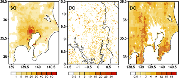
Figure 1. The prior fields of (A) fossil fuel emissions of January 2018 from ODIAC, (B) biomass burning emissions of January 2018 from GFAS, and (C) GPP of April 2018 from Zeng et al (2020b). Fluxes are downscaled from original datasets to model resolution of 0.025° × 0.025°. (A), (C) shows the Tokyo region and (B) shows the African country Ghana. Units in g C m–2 d–1.
Download figure:
Standard image High-resolution imageThe CO2 mole fractions from the sites of urban CO2 observation projects in the USA, Japan, and Europe and observations from background sites were also used in this study (supplementary figure 1 shows the location of sites included in the inversions). The data sources include the National Institute of Standards and Technology (NIST) Northeast Corridor; NEC (Karion et al 2019, 2020), Los Angeles Megacity Carbon Project network (hereafter L. A.; Verhulst et al 2017, Kim et al 2021), Salt Lake City CO2 measurement network, Indianapolis Flux Experiment (INFLUX Davis et al 2017, Miles et al 2017, Richardson et al 2017), Atmospheric Carbon and Transport—America (ACT–America; Miles et al 2018, Wei et al 2021), China Meteorological Administration (CMA), World Data Centre for Greenhouse Gases (WDCGG), National Institute for Environmental Studies (NIES), European Integrated Carbon Observation System (ICOS), and Observation Package–CO2 (ObsPack–CO2) GLOBALVIEWplusV7.0 (Schuldt et al 2021). The observations under the NOAA aircraft program (available in ObsPack) and Comprehensive Observation Network for TRace gases by AIrLiner (CONTRAIL) (Machida et al 2018) were used as an independent dataset for validating the optimized fluxes. These data were not included in the inversion analysis. Details on the downscaling of prior fluxes, preparation of prior uncertainty, surface CO2 observations and aircraft observations are given in supplementary note 2. Additional details on observation sites are in supplementary tables 2 and 3.
2.1. Tracer transport modeling
A coupled transport model was used to simulate CO2 transport at high resolution. The CO2 mixing ratios from the above-mentioned urban areas and background sites, along with the meteorological parameters from JRA-55 reanalysis data were used in Lagrangian model FLEXPART v.8.0 (Stohl et al 2005) to prepare the surface flux footprints on a 0.025° × 0.025° grid. These footprints are consistent with each observation and are produced from the model run in a backward mode. The 3D concentration field and the surface flux footprint from FLEXPART model are then coupled to the Eulerian model within a coupling time of 2–3 d before each observation event and are mapped to NIES-TM model grids (5° × 5° resolution). The Eulerian model is run in forward mode to obtain the surface flux corresponding to the simulated concentrations. The sum of concentrations from the Eulerian and Lagrangian model gives the total concentration. More details on the procedure are given in supplementary note 3.
2.2. Inverse model and the experiment setup
We use a combination of the coupled transport model NIES–TM–FLEXPART with the variational optimization algorithm (Maksyutov et al 2021), which constitutes the inverse modeling system NIES–TM–FLEXPART–VAR (NTFVAR or NIES–TM–FLEXPART–variational). The inversion algorithm was tested by Maksyutov et al (2021) for the problem of finding the best fit to the CO2 observations provided by the ObsPack dataset by optimizing the corrections to the terrestrial biosphere and ocean fluxes. These optimized fluxes were compared to other CO2 inverse models in an intercomparison study by Byrne et al (2023) using practically the same base prior flux set as in this study. But this model was modified to optimize fossil fuel emissions additionally. The horizontal flux correlation distance was kept at 100 km, as the study focuses on the subnational/regional scale fossil emissions. Further details are available in supplementary note 3.
Two sets of inversions were carried out from 2015 to 2019. In the first set (optimizing two flux categories), only the fluxes corresponding to terrestrial-biosphere and ocean–atmospheric exchanges (natural fluxes) were optimized. Whereas, in the second set (three flux categories) of inversions, fossil fuel fluxes were optimized in addition to natural fluxes for investigating the added benefit of optimizing fossil fuel emissions in representing the urban CO2 concentrations. The high-resolution prior fluxes (0.025° × 0.025°) utilized in the inverse model were also tested by changing the model parameters, including horizontal flux covariance distance and prior flux uncertainty. Here, we present the results from two cases with different uncertainties; base case (C1; prior fossil fuel flux uncertainty set to 30% of monthly climatology) and with flux uncertainty inflated by a factor of 1.5 (C2; prior flux uncertainty set to 45%).
To estimate flux errors, a set of inversions were conducted for the year 2018 with case C2 using the ensemble of pseudo datasets of terrestrial ecosystem respiration (RECO) fluxes, fossil fuel fluxes, and observations as described in Chevallier et al (2007). They were prepared by adding random noise to the datasets. The uncertainty in the posterior fluxes is estimated as the standard deviation of the posterior flux ensemble. Finally, the evaluation of the model with independent datasets was carried out using a set of aircraft observations in prior and posterior forward simulations.
3. Results
As we are focusing in this study on the emissions from fossil fuels, the improvements in additionally optimizing fossil fuel fluxes (three-category inversion) are compared to the results from optimizing only natural fluxes. The relative error (in percentage) of concentrations from the two sets of inversions were compared (supplementary figure 2). The corrections from three category inversions were found to be 1%–3% higher at many sites of Indiana and across the NEC network (21 sites), with slightly higher corrections on a few sites for case C1, while the sites in Los Angeles have got the highest correction of 9%–12%. Over Germany, France, and England, the optimized corrections were in the 1%–3% range, for both cases C1 and C2. From the results, it was found that the present model could effectively reduce root mean square error (RMSE) in simulated concentrations by additionally optimizing fossil fuel fluxes. Hence, the results are discussed only for the three category inversions for the two cases C1 and C2.
3.1. Optimized natural fluxes and comparison to CarbonTracker and OCO2-MIP
The results from the natural fluxes are evaluated for the 22 TransCom-3 regions (Baker et al 2006). The optimized terrestrial biosphere fluxes are mainly contributed from tropical Asia and America (supplementary figures 3(a) and (b)), whereas the optimized values over tropical oceans are small compared to other regions. Generally, the annual net fluxes from NIES model are within the multi-model spread when compared to other models (supplementary figures 4(a) and (b)) in the OCO2-MIP (Baker et al 2023). Such divergence of regional fluxes can be the manifestation of the transport model differences. In most cases it is difficult to assign which process is responsible when deviations from the model mean or median are noticeable, like for Boreal North America or Temperate Eurasia, where our model still does not disagree with the range of alternative estimates of land sinks (Deng et al 2022). Some impact of strong prior ocean sink may drive land fluxes higher in Australia. Better understanding of the processes responsible for differences in the estimated fluxes can be achieved by analyzing the fluxes in connection with the simulation of reference tracers like SF6, radon (Krol et al 2018) and COS (Remaud et al 2023).
The large-scale net flux estimates were evaluated by comparing the mean monthly optimized fluxes with CT2019b fluxes. The optimized fluxes are found to represent the seasonal cycle well and their magnitudes over the land regions have similar variations as in CT2019b (figure 2). The fluxes over Northern America and Europe (Regions 1, 2, and 11) are well constrained by the observations, and therefore have a reasonable agreement between the models, whereas the summer variations over the Asian Tropical (Region 9) region are not well captured by the model, as can be seen from the spread of the estimates. For ocean fluxes, the posterior is not significantly different from the prior, except for the Southern Ocean and North Pacific Temperate regions. The ocean flux uncertainty values are seemingly too tight to adjust the oceanic flux, while the model chooses to adjust the land fluxes that have larger uncertainties. Hence the ocean flux corrections are mostly insignificant. However, since the focus of this study is on fossil fuel flux estimates, the weights of relative adjustments to land and ocean fluxes are less important.
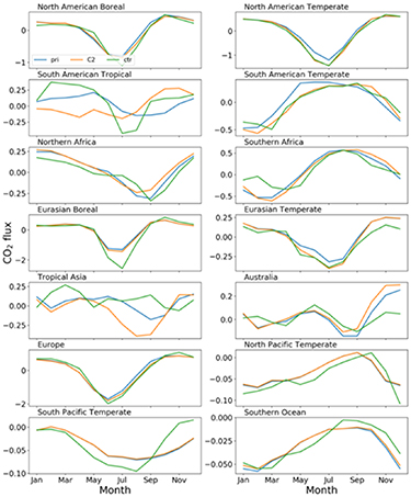
Figure 2. Mean monthly prior (pri) and optimized fluxes of C2 (model) case for the terrestrial biosphere and ocean–atmosphere exchanges along with the fluxes of CT2019b (ctr). Units in gC m–2 d–1.
Download figure:
Standard image High-resolution image3.2. Estimated fossil fuel fluxes and evaluation with regional inventories
The annual mean maps of (averaged over the period 2015–2019) posterior fossil fuel flux are shown in figures 3(A) and (B). One of the distinct features of the model is the use of high-resolution uncertainty data along with the smoothed scaling factors, by which the model picks up the finer scale features of fluxes in the estimation of flux corrections. Although the horizontal covariance length is chosen to be 100 km, the corrections are found to coincide with the regions of higher anthropogenic activities (figures 3(A) and (B)), such as the USA, Europe, and Asian countries (mainly Japan, China, and India). The spatial patterns are well represented over regions with numerous observations, especially in the U.S.'s urban areas such as Indiana, Colorado, Connecticut, and New York. But the difference between the optimized fluxes between two cases, C1 and C2 shown in figure 3(C), indicates that the estimated fluxes from case C2 was higher than C1 except over California, Northeastern states of America, and Northwest Italy.
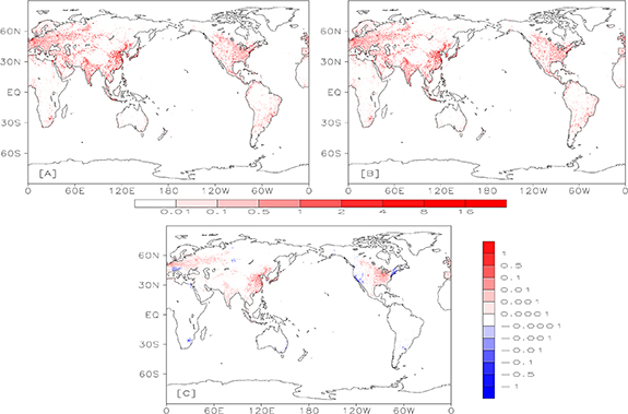
Figure 3. Annual mean posterior fossil fuel CO2 flux averaged over 2015–2019 for (a) C1, (b) C2 and (c) the difference between C2 and C1 in units of gC m–2 d–1.
Download figure:
Standard image High-resolution imageThe estimated fossil fuel fluxes were also evaluated regionally. For which, the subnational/regional scale fossil fuel CO2 fluxes were compared against inventories for selected states in the U.S., countries in the U.K., and the E.U., where alternatives to prior regional fossil fuel emission inventories are available. It would be interesting to have flux estimates at a larger scale, like the U.S., but the top-down fossil emission estimate is likely to be more uncertain at such a scale, as observation coverage is sparse over many important regions with considerable emissions. The annual estimated fossil fuel fluxes for 2015–2018 are compared with the EPA inventory, as the U.S. EPA updates the inventory regularly and it is the authority to report the U.S. GHG emissions to the UNFCCC (Basu et al 2020). The ratio of EPA and optimized fluxes (C1, C2) to ODIAC are shown in (figure 4(A) and (B)). The model-estimated fossil fluxes show better agreement with the state-level estimates of EPA. We consider this as an impact of using urban measurements in the inversion system as these estimates are constrained by the numerous urban observations, which are usually not included in global inversions. This is obvious over the states of Indiana, New York, Massachusetts, Connecticut, Maryland, and Virginia, which are mainly covered by the NEC and INFLUX network. The only difference between cases C1 and C2 is over the state of Wyoming. The estimates over the east coast and the west coastal regions are well constrained by the observations. However, the discrepancy between EPA and model estimates over the southcentral coast could be due to insufficient measurements over the region.
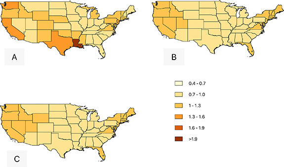
Figure 4. The ratio of CO2 emissions from (a) EPA to ODIAC, (b) optimized C1 to ODIAC, and (c) optimized C2 to ODIAC over the states of the U.S.
Download figure:
Standard image High-resolution imageFigure 5(a) shows the state-wide fossil fuel emission estimates for selected states/regions along with uncertainty values. The optimized values are higher than the prior, attaining a correction in the right direction for California, Massachusetts, New York, Connecticut, Virginia, and Maryland. The estimates from case C2 for California, New York, and Virginia are closer to EPA inventory, whereas, over Maryland and Connecticut, the estimates were not very different for C1 and C2 cases. The prior over the state of Indiana was 7% higher than the EPA inventory, but on optimization, the estimates were closer to EPA (less by 7%) inventory with enhanced corrections from case C2 (46.97 Tg C yr–1) compared to case C1 (44.20 Tg C yr–1). Over California, the estimates are 33% lower than the EPA inventory, partly contributed by the lower emissions from ODIAC (Hedelius et al 2018) and the model's difficulty in capturing seasonal variations over the region. Comparisons with similar regional studies (supplementary note 4) and estimates are available in supplementary table 4.

Figure 5. Comparison of prior, posterior (C1 and C2), and inventory data of (EPA/TNO–CAMS) fossil fuel fluxes (Tg C yr–1) for the selected states of (a) USA and (b) countries of the E.U. and the U.K. The uncertainty estimates of case C2 for the year 2018 are also shown.
Download figure:
Standard image High-resolution imageThe annual mean fossil flux estimates for selected countries of the E.U. are compared to the inventory from TNO–CAMS (figure 5(b)). The inventory for the most recent available year, 2014, was used. Positive corrections are obtained over the U.K. and France, but the adjustments are not sufficient for the posterior to match the TNO data and hence the estimates are less than the inventory. Flux corrections for individual countries in the U.K. suggest emissions closer to the inventory than the prior emissions. Over Germany, the posterior is less than the prior, resulting in a lower estimate than inventory. The estimates for selected E.U. countries are given in supplementary table 4. The estimation of posterior flux uncertainty is carried out for the year 2018, but only for case C2, due to its improved performance over most of the regions.
3.2.1. Uncertainty estimates of posterior fluxes
The uncertainty analysis reveals that the posterior uncertainty is less over the regions where dense observations are available. Over USA (figure 5(a)), the uncertainties are high over Indiana and California, which could be due to the strong influence of vegetation and large fossil flux correction from prior (ODIAC), respectively. However, for the two cases, C1 and C2, the spread of flux estimates is within the uncertainty values. On average, the flux corrections (chi-square of 1.22 over U.S.) for several U.S. regions appear somewhat larger than the posterior uncertainties (estimated as the spread of posterior ensemble fluxes), which could indicate the need for revising the method of posterior uncertainty estimation.
3.3. Comparison of prior and optimized forward simulations with observations
The time series of optimized, forward, and observed concentrations for sites dominated by natural fluxes as well as fossil fuel emissions were examined to check the ability of the model to represent the seasonal variability. The seasonal changes of selected sites such as Syowa (SYO), Pallas (PAL), Lampedusa (LMP), and Hyytiälä (SMR) are dominated by natural flux (N.F.) and Arlington_VA (ARL), Norunda (NOR), Stockholm_NJ (SNJ) and Trainou (TRN), are sites dominated by urban CO2 emissions (F.F.). The seasonal variations at these sites are well represented by the model, and the optimized model show (supplementary figure 5) clear improvements compared to prior in simulating observed concentrations irrespective of their location. The RMSE and bias for the prior and optimized forward for the cases C1 and C2 for representative sites are given in supplementary table 5. The model performance for all the sites in the urban network is discussed using the statistics RMSE and bias for cases C1 and C2 (figure 6). The RMSE is found to have decreased relative to the prior, and the values of bias are close to zero. But a few exceptions are noticed, especially over California with large negative bias and higher posterior RMSE. The reduction in the posterior bias is contributed by the bias reduction from the natural as well as fossil fuel flux components. However, over California the bias from natural fluxes is reduced considerably, but there seems no contribution from fossil fluxes. The bias correction seemed to be appreciable only in some of the background sites and not over the urban sites of California. Since the variability over this region is poorly captured by the model, the model misfit and bias are high. This may be partly due to complex topography, wind patterns and the lower prior fluxes (ODIAC) supplied to the model. The higher bias in sites of California is also reported by Brophy et al (2019). They explain the bias is high during Oct-Nov months and showed that highest bias is noticed at CIT. In this study the urban sites such as CIT, FUL, FRA, US2, US1 and ONT have high bias, of which CIT has got the highest bias.
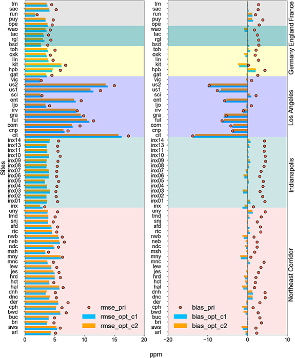
Figure 6. RMSE and bias of prior (red dots) and optimized simulations for the sites from megacity projects for the cases C1 (blue bars) and C2 (orange bars). Stations are grouped based on the representing region demarcated by unique background color and are labeled on the right side of the figure.
Download figure:
Standard image High-resolution imageThe coefficient of determination (r2) between the prior forward and observation was found to be 0.71, which has increased to 0.77 (C1) and 0.79 (C2) for optimized simulations. The statistics for all sites in urban networks are given in supplementary table 6. The RMSE for the sites in urban network (except Los Angeles) was reduced to 4.8 ppm from 5.15 ppm and the bias reduced to −0.20 ppm from 1.29 ppm on optimization.
To interpret the regional difference in the CO2 emission estimates, the analysis is extended to three subcontinental regions of the USA, U.K. and E.U. Over the USA, the site of Indiana shows a good model to observations fit, with an average RMSE of 3.84 for case C1 (3.74 for case C2) ppm of 0.033 (–0.03) ppm. Over Connecticut, the RMSE and bias are 4.71 (4.64) and –0.27 (–0.32 ppm), respectively. But over California, though higher RMSE is obtained, there is still an improvement from the prior. The time series plots of prior, posterior simulations, and observations for the regions of study are shown in supplementary figures 6–8.
Over Japan, only two data sites are present: Kisai, Saitama (KIS) and Tokyo (TOK), with sparse data. For KIS (supplementary figure 9), the prior RMSE of 6.52 ppm reduced to 6.46 (6.49) ppm, whereas the prior bias of −0.98 has become stronger [–2.34 (–2.44) ppm for cases C1 and C2 respectively]. The mean RMSE and mean bias for selected countries of the U.K/ the E.U. (details in supplementary table 7) are; for England 3.13 for case C1 (3.07 for case C2) and −0.22 (−0.17), for Germany 4.32 (4.27) and −0.18 (−0.20); for France 3.38 (3.34) and 0.46 (0.45) respectively. The time series plots are given in supplementary figures 10–12. It is to be noted that the seasonal variations are well represented, and the simulated concentrations are in good agreement with the urban observations.
3.4. Model evaluation using independent observations
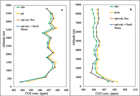
To evaluate the inverse model, an independent set of aircraft data was utilized along with the prior and optimized fluxes to obtain the simulated CO2 concentration. The concentration obtained from the simulations of the prior and posterior forward model for optimized natural fluxes (opt-nat. fluxes) as well as for natural and fossil fluxes (opt-nat. + fossil fluxes) were averaged and compared with observations at every 300 m altitude over the U.S. and for every 500 m over the U.K. and the E.U. (figures 7(a) and (b)). The simulations are carried out only for the C2 case due to its better performance compared to C1 case. The optimized model shows (figure 7(a)) clear improvements over the prior and is closer to the observations for the entire vertical column up to 5 km altitude. The prior concentrations (simulated with prior fluxes) were higher by around one ppm than the observations, which was adjusted by the model to obtain a better agreement of optimized values with the observations. Over the U.K. and the E.U. corrections from the prior are noticeable and the model estimates are closer to observed concentrations. The model reduced the higher concentrations of prior (∼1.2 ppm) to obtain the optimised values. Up to 3000 m, stronger corrections are observed which is being reflected from the seasonal pattern for the spring and winter. It is to be noted that optimizing the fossil fluxes additionally to biogenic/natural ones produces only a minor impact on the model fit to observations in the vertical profile (figure 7). This can be explained by the biogenic fluxes being several times stronger over large regions than the fossil fluxes especially in summer leading to a dominant role of land biogenic fluxes in reducing the model-observations misfit. While the corrections to the fossil signals are noticeable near urban sources, the impact of biogenic fluxes is significantly stronger elsewhere.
Figure 7. The vertical profile of observations (obs), prior forward (pri), forward simulations with optimized natural fluxes (opt- nat. flux) and forward simulations with optimized natural and fossil fluxes (opt- nat. + fossil flux) using independent aircraft observations over the U.S. (a), the U.K. and the E.U. (b) The data are averaged for every 300 m/500 m altitude bins respectively. An offset 0.6/0.8 ppm is subtracted from the respective prior concentration to show the improvements of the optimized profile from prior.
Download figure:
Standard image High-resolution image
4. Discussion
The top-down approach based on atmospheric observations is a promising tool to estimate GHG emissions at a national/subnational scale as it can effectively use the atmospheric GHG observations. Several developments at regional scale inversions successfully separate the fossil fluxes from natural fluxes and provide reasonable fossil emission estimates based on the measurements from an urban network. But, at a larger scale, the carbon budget is estimated by considering fossil emissions as a known quantity and the natural fluxes are estimated by subtracting the prior fossil emissions from the posterior. However, this approach will leave a residual of fossil emissions in the posterior (Oda et al 2019, Wang et al 2020), in addition to the errors from top-down methods (Chevallier et al 2006, Angevine et al 2020). Therefore, measurements from a denser observation network and a high-resolution inverse model are required for resolving fluxes at higher spatial scales and achieving a robust estimation of natural and fossil fluxes. The cost in setting up a denser network and resources required for such a high-resolution model remains a challenge.
In this study, a high-resolution global CO2 inverse model was used and its capability in estimating subnational/regional scale CO2 emissions, using all available ground measurements was examined and discussed. While previous research works in the field are concentrated at continental or national scale, this study is an exception by employing a global model to estimate CO2 emission at a regional scale. Furthermore, the existing regional inversion studies to estimate fossil emissions are limited to smaller regions/countries of interest (Lauvaux et al 2020, Lian et al 2023). The recent inversion intercomparison studies (Deng et al 2022, Byrne et al 2023) also supports this argument. Thus, the concept of using high-resolution global inversion model to estimate regional (province-scale/country) natural and fossil emissions (CO2 budget) is first-hand. Additionally, large-scale Bayesian inversions are limited with the use of selected background measurements, but this inversion system can use all measurements (surface/satellite) of the globe to disseminate CO2 emission estimates.
The emission estimates from this model are optimized separately to comprehend the contributions from each flux category and the model is successful in reproducing the seasonal cycle at all background sites and most urban areas of North America and Europe. Though the natural fluxes are large or comparable to fossil emissions at sites like ICOS or NOAA-ESRL (Levin and Karstens 2008, Shiga et al 2014), in the present study the observations are taken closer to the sources by the urban networks in order to avoid weakening of the fossil signal by horizontal mixing. Thus, the signals of fossil emissions can be separated from natural fluxes by using the measurements from regional networks. In addition, a reasonable agreement of category-wise flux estimates with regional independent inventories imply that the estimated fluxes are well constrained by observations in urban regions. The evaluation with independent aircraft data also confirms that the overall flux adjustments are in the desired direction.
5. Conclusions
The present study demonstrates the use of a global high-resolution inverse model to estimate CO2 budget at subnational scale by utilizing the regionally available ground measurements. This approach suggests a promising way to independently evaluate national/subnational emission inventories. The biospheric flux estimates from the model are comparable to established models and the estimates of fossil emissions are comparable to the reference estimates from regional inventories over Europe and the U.S. The estimates from the inverse model are constrained by measurements in urban areas with dense observations and the flux adjustments are verified using an independent observation. We demonstrated that for many the U.S. states, fossil flux corrections at least partially compensate for the difference between prior (ODIAC) and reference (EPA) emission datasets.
The inverse model can be tuned further with the inclusion of high-resolution meteorological drivers and satellite CO2 data that would enable flux corrections over data-sparse regions in the global surface observation network. Further improvements in the transport model simulations (mostly FLEXPART) should also improve flux estimates from the model. Thus, the proposed inverse modeling system is a promising tool to independently assess fossil emissions at desired scales by using numerous atmospheric observations and thereby considered as a step towards a system to regularly monitor emissions and, eventually, their trends.
Acknowledgments
All simulations for this work were carried out in the Supercomputer System at National Institute for Environmental Studies, Japan. Authors (LRN, RJ, SM, and TM) acknowledge support from the GOSAT project funding.
We thank all the data providers of megacity projects for collecting CO2 data for several years—N Miles, S Richardson, and K J Davis (PSU) for the data over Indianapolis through the Indianapolis Flux Experiment (INFLUX) project; A Karion (NIST) for the valuable comments to improve the manuscript and for the observations over Northeast Corridor; J J Kim (NIST) for the CO2 data from Los Angeles through Los Angeles Megacity Carbon Project; L E Mitchell and J C Lin (U–ATAQ) for the measurements from Salt Lake City, Utah (HDP, UTMSA, UTDBK, UTMUR, UTRPK, UTSUG, UTUOU) through Salt Lake City CO2 measurement network.
We are grateful to D Kubistin, (DWD) and colleagues for gathering CO2 data from several sites (GAT, KIT, LIN, OXK, STE, TOH) of ICOS Germany; M Ramonet for the observations from the sites (OPE, PAL, SAC, TRN) of ICOS France and for the valuable contributions to ICOS collection from J Hatakka (FMI); S M Platt (NILU); P Cristofanelli (ISAC–CNR); K Komínková (CAS); Martine De Mazière (OPAR); P Marklund (FEM, SLU); G Manca (EC–JRC), L Emmenegger (Empa); B Scheeren of (RUG), I Lehner (LU); A Colomb (LSCE), J Levula (UHELS). We thank Y Terao (NIES) and S Ishidoya (AIST) for CO2 observations at Tokai University in Yoyogi, Tokyo, Y Muto for collecting the data at Kisai, Saitama, distributed by WDCGG.
We appreciate the contributors of Obspack data product provided by NOAA/ESRL: A Manning and Grant Forster (UEA); A Hensen, A Frumau, D van Dinther, Pim van den Bulk (ECN); A Vermeulen (L U); A Andrews (NOAA); D Jaffe (UofWA); John Lee (UofME); B Viner (SRNL); Stephan De Wekker (UofVA); M L Fischer of (LBNL); Peter Bakwin (NOAA); B Law and C Hanson (OSU); B Stephens (NCAR), C Labuschagne and W Joubert (SAWS); C L Myhre and O Hermanssen (NILU), C Sweeney, J B Miller (NOAA); C E Miller (NASA–JPL); J Turnbull (GNS), A Karion (NIST) and K McKain (NOAA); Francesco Apadula (RSE); F Meinhardt (UBA–SCHAU); G Brailsford and S Nichol (NIWA); H Meijer, H Chen and B Scheeren (RUG); I Levin, S Hammer and J D Coletta (UHEI–IUP); J Levula, P Keronen and P Kolari (UHELS); O Peltola (FMI); J Necki, M Galkowski, M Zimnoch, L Chmura and J Bartyzel of (AGH); Josep–Anton Morgui, R Curcoll and S Climadat (ICTA–UAB). We acknowledge Ed Dlugokencky (NOAA) for contributing flask data from several sites and Doug Worthy (ECCC) for the surface in-situ data of Canada. We thank K Saito (JMA); K Thoning and Pieter Tans (NOAA); L Haszpra (RCAES); L V Gatti of (INPE); M Delmotte, M Ramonet and G Bentz (LSCE); M Leuenberger (KUP) and L Emmenegger (Empa); M Molder (LUND–NATEKO); N Mihalopoulos (ECPL); O Laurent (ICOS–ATC); F Gheusi (OMP) and T Machida (NIES); P P Rivas, E Cuevas, Enrique Reyes–Sanchez, R Ramos and Vanessa Gomez–Trueba (AEMET); R Keeling, L Merchant, S Clark and E Morgan, S Piper, A Cox, S Walker, Bill Paplawsky (SIO); E Hintsa (NOAA); R Langenfelds, P Krummel and Zoe Loh of (CSIRO); S Newman (CIT); S C Biraud (LBNL–ARM) and M Torn (LBNL); S Aoki, S Morimoto (T U) and Daisuke Goto (NIES); A Manning (Met Office); S O'Doherty, D Young and D Say (UNIVBRIS); S Wofsy and M Sargent (H U); Tim Griffis of (UMINN). We are grateful to N Miles, S Richardson, and K J Davis (PSU) for the data from AMERIFLUX project; J Hatakka and T Aalto (FMI) for the data from the site Pallas, Finland (PAL) distributed by WDCGG.
We are thankful to S Fang (CMA) for the hourly in situ dataset from three CMA sites (LIN, LNA, SDZ) in China. We acknowledge the use of CarbonTracker model outputs and thank A Jacobson and other members of the group for their contributions to this data.
We acknowledge the use of GFAS data; 'GFAS data was generated using Copernicus Atmosphere Monitoring Service Information 2021' and 'neither the European Commission nor ECMWF is responsible for any use that may be made of the information it contains'.
The aircraft observations from the CONTRAIL dataset have also been utilized. The authors thank Toshinobu Machida and colleagues for their effort to collect and distribute this dataset for research purposes. Besides, the v10 OCO2-MIP flux datasets were used in this study. The authors appreciate the valuable contributions of Brendan Byrne and others for making the flux datasets freely available for research studies.
Data availability statements
All data that support the findings of this study are included within the article (and any supplementary files). The links to the dataset are given below.
Prior fluxes
Biomass burning—https://confluence.ecmwf.int/display/CKB/CAMS%3A+Global+Fire+Assimilation+System+%28GFAS%29+data+documentation
ODIAC (version 2020)—www.nies.go.jp/doi/10.17595/20170411.001–e.html
Ocean Flux—www.nies.go.jp/doi/10.17595/20201020.001–e.html
Vegetation uptake, respiration—www.nies.go.jp/doi/10.17595/20200227.001–e.html.
CO2 Observations
China—https://data.mendeley.com/datasets/w3bwmr6rfg/1
ICOS—http://icos-cp.eu/data-products/atmosphere-release
INFLUX—http://doi.org/10.25925/20210801
ACT–America—http://doi.org/10.25925/20210801
NIES—www.nies.go.jp/doi/10.17595/20210510.003–e.html
NIST–Los Angeles—http://doi.org/10.18434/mds2–2388
NIST—Northeast Corridor—https://data.nist.gov/od/id/mds2–2491
Obspack—http://doi.org/10.25925/20210801.
Salt Lake City—http://doi.org/10.25925/20210801, http://doi.org/10.7289/V50R9MN2
WDCGG—https://urn:x–wmo:md:jp.go.jma.wis.dcpc–wdcgg::0065–2017–1001–01–01–9999
https://gaw.kishou.go.jp/search/file/0065-2017-1001-01-01-9999
CONTRAIL—http://doi:10.17595/20180208.001
Inventories
EPA (2020)—www.epa.gov/statelocalenergy/state–co2–emissions–fossil–fuel–combustion
TNO–CAMS—10.5281/zenodo.112889.
Model comparison
CT2019—http://ftp://aftp.cmdl.noaa/gov/products/carbontracker/CT2019B/
OCO-2 v10 MIP gridded fluxes IS—https://gml.noaa.gov/ccgg/OCO2_v10mip/.
Funding information
This research is funded by the GOSAT Series Project of NIES, Japan and Progetto nazionale Rafforzamento del Capitale Umano CIR01_00019 – PRO – ICOS – MED for Pamela Trisolino.
Conflict of interest
The authors have no competing interests that might influence this research work.
Author contributions
Contributed to conception and design: S M
Contributed to acquisition of data: L N, R J, S M
Contributed to analysis and interpretation of data: L N, R J, S M, T O
Drafted and/or revised this article: L N, R J, S M, T O, P T, J Z, J W K, T M
Approved the draft for submission: L N, R J, S M, T O, P T, J Z, J W K, T M.
Supplementary data (8.2 MB PDF)