

Abstract
Anthropogenic changes in the variability of precipitation stand to impact both natural and human systems in profound ways. Precipitation variability encompasses not only extremes like droughts and floods, but also the spectrum of precipitation which populates the times between these extremes. Understanding the changes in precipitation variability alongside changes in mean and extreme precipitation is essential in unraveling the hydrological cycle's response to warming. We use a suite of state-of-the-art climate models, with each model consisting of a single-model initial-condition large ensemble (SMILE), yielding at least 15 individual realizations of equally likely evolutions of future climate state for each climate model. The SMILE framework allows for increased precision in estimating the evolving distribution of precipitation, allowing for forced changes in precipitation variability to be compared across climate models. We show that the scaling rates of precipitation variability, the relation between the rise in global temperature and changes in precipitation variability, are markedly robust across timescales from interannual to decadal. Over mid- and high latitudes, it is very likely that precipitation is increasing across the entire spectrum from means to extremes, as is precipitation variability across all timescales, and seasonally these changes can be amplified. Model or structural uncertainty is a prevailing uncertainty especially over the Tropics and Subtropics. We uncover that model-based estimates of historical interannual precipitation variability are sensitive to the number of ensemble members used, with 'small' initial-condition ensembles (of less than 30 members) systematically underestimating precipitation variability, highlighting the utility of the SMILE framework for the representation of the full precipitation distribution.
Export citation and abstract BibTeX RIS

Original content from this work may be used under the terms of the Creative Commons Attribution 4.0 license. Any further distribution of this work must maintain attribution to the author(s) and the title of the work, journal citation and DOI.
1. Introduction
Anthropogenic changes in the variability of precipitation stand to impact both natural and human systems in profound ways, from enhancing volatility of crop yields and dryland productivity (Rowhani et al 2011, Gherardi and Sala 2019), which renders vulnerable populations and livestock (Shively 2017, Sloat et al 2018), to enhancing flood risk and damage (Nobre et al 2017). Changes in mean or extreme precipitation alone are not the only drivers of shifts in the distribution of hydrometeorological events. The 'space between' mean and extreme also determines the properties of the distribution. Precipitation variability connects the times between dry and wet periods, between droughts and floods. Scientific understanding and projection of such changes in the hydrological cycle, including understanding of the uncertainties inherent to their manifestation, is therefore critical for informing policy and management decisions aimed at mitigating and/or adaption to imminent hydrometeorological threats.
There is scientific consensus that mean precipitation is changing with warming globally at a rate of about 2% K−1 (Allen and Ingram 2002, Allan et al 2020), driven by an increase in moisture but constrained by radiation cooling. Heavy precipitation (99.9th all-day percentile of daily precipitation) is increasing at a rate of around 7% K−1 globally, mainly driven by the change in near surface moisture (O'Gorman and Schneider 2009). At local scales, these rates can be higher due to changes in dynamics (Lenderink and van Meijgaard 2008, Berg et al 2009, Westra et al 2014, Lenderink et al 2017, Wood and Ludwig 2020). It is however not settled whether the change in precipitation variability with warming follows the change of mean precipitation or the rate of near surface moisture. Pendergrass et al (2017) have argued that precipitation variability changes globally above the rate of mean precipitation, but below the rate of heavy precipitation. The physical processes leading to changes in mean and extreme precipitation, as well as variability can thereby be different (Bintanja et al 2020, van der Wiel and Bintanja 2021). Changes in variability are commonly studied on regional scales, for example the Asian Monsoon regions (Brown et al 2017a), the North American Monsoon (Dong et al 2018), or the Arctic (Bintanja et al 2020). Earlier studies have shown an increase in interannual variability to be strongest in the tropics and mid-latitudes (Boer 2009, Seager et al 2012, He and Li 2019). However, most work has focused on variability changes related to changes in El Nino-Southern Oscillation (ENSO) (Maher et al 2018, Haszpra et al 2020).
Quantification of anthropogenic changes in the distribution of precipitation is challenged by the ever-present influence of internal climate variability. Internal variability in the climate system is an irreducible and important source of uncertainty induced by natural processes in the atmosphere-ocean-land-biosphere-cryosphere system (Hawkins and Sutton 2009, Deser et al 2012, Lehner et al 2020). It is difficult to account for internal variability in a single climate model simulation, because it can only show a limited number of possible weather and climate events. This limitation holds true for the observational record as well. The current best-practice to robustly estimate the model's forced response and its internal variability is by using long control simulations or large ensembles (Brown et al 2017b, Maher et al 2018, Milinski et al 2020). Although, progress is being made on isolating internal variability in individual simulations and observations using statistical methods (Smoliak et al 2015, Deser et al 2016, Sippel et al 2019, Wills et al 2020). However, long control simulations cannot account for forced changes in internal variability in a changing climate. Large ensembles are multi-member climate simulations using a single climate model under the same external forcing (i.e. radiative forcing), applying perturbations at the initialization of each member, which will create diverging climate trajectories. These ensembles can be described as single-model initial-condition large ensembles (SMILEs, for examples see Kay et al 2015, Maher et al 2019). While multi-model archives with mainly single or only a limited number of members, such as the Coupled Model Intercomparison Project (CMIP) phase 5, confound structural uncertainty (differences in model formulation) with those from internal variability, archives of multiple SMILEs are well suited to address both sources of uncertainties. Within CMIP, internal variability accounts for roughly half of intermodel spread for projected changes in precipitation over North America and Europe over the next 50 years (Deser et al 2020 and references therein). Also, changes in large scale dynamics, such as ENSO, which itself drive interannual variability in surface climate variables, often show a small signal-to-noise ratio, such that large ensembles are needed to robustly compute their variance and its change (Maher et al 2018, Milinski et al 2020).
Disentangling forced changes in variance from natural variance, particularly at decadal timescales, is statistically untenable with a single climate realization, because of their small sample size, but achievable through using SMILEs, due to their large sample size. Further, SMILEs enable a more robust model evaluation by providing more complete information on biases (Maher et al 2019, Suarez-Gutierrez et al 2020). There are now a growing number of SMILEs stored in public archives (Deser et al 2020), affording more multi-SMILE studies (Maher et al 2020, 2021, Schlunegger et al 2020).
Here, we use six state-of-the-art fully-coupled global SMILEs with daily data from the Multi-Model Large Ensemble Archive (MMLEA; Deser et al 2020) to quantify changes in precipitation (mean and extreme) and its variability on timescales from annual to decadal under the Representative Concentration Pathway 8.5 (RCP8.5) scenario. The usage of multiple SMILEs enables us to answer the question whether and where changes in variability are robust and whether different models agree on these changes. We use a simple evaluation framework for interannual precipitation variability in SMILEs and analyze to what extent ensemble size influences the representation of variability.
2. Data
2.1. Large ensembles
We make use of six publicly available SMILEs with daily precipitation data, and one SMILE with monthly data (MPI). These SMILEs constitute a reliable representation of the CMIP5 ensemble (Lehner et al 2020, Maher et al 2021) and the individual models are largely structural independent (Knutti et al 2013, Sanderson et al 2015). All SMILEs follow standard CMIP5 'historical' and RCP8.5 forcing protocols. The strong forcing scenario allows for the analysis of changes across a broader range of climate sensitivities, allowing for a more robust separation of internal versus model uncertainty. The models range from ∼2.8° to ∼1.0° horizontal resolution and from 16 to 100 ensemble members. In terms of initialization, the models used either Micro, Macro, or both schemes (Hawkins et al 2016). For detailed model specifications and experimental design, the reader is referred to the references in table 1.
Table 1. Single-model initial-condition large ensembles (SMILEs) used in this study.
| Modeling center | Model version | Resolution (atm ocn−1) | Initialization (methods) | No. of members | Reference |
|---|---|---|---|---|---|
| CCCma | CanESM2a | ∼2.8° × 2.8°/∼1.4° × 0.9° | Macro and Micro | 50 | Kirchmeier-Young et al (2017) |
| NCAR | CESM1a | ∼1.3° × 0.9°/nominal 1.0° | Micro | 40 | Kay et al (2015) |
| CSIRO | MK3.6a | ∼1.9° × 1.9°/∼1.9° × 1.0° | Macro | 30 | Jeffrey et al (2013) |
| SMHI/KNMI | EC-Eartha | ∼1.1° × 1.1°/nominal 1.0° | Micro | 16 | Hazeleger et al (2010) |
| GFDL | CM3a | 2.0° × 2.5°/1.0° × 0.9° | Micro | 20 | Sun et al (2018) |
| GFDL | ESM2Mb | 2.0° × 2.5°/1.0° × 0.9° | Macro | 30 | Rodgers et al (2015) Schlunegger et al (2019) |
| MPI | MPI-ESM-LRa,c | ∼1.9° × 1.9°/nominal 1.5° | Macro | 100 | Maher et al (2019) |
aDaily outputs are available on the Multi-Model Large-Ensemble Archive (MMLEA): www.cesm.ucar.edu/projects/community-projects/MMLEA/. bDaily outputs are available on the Princeton Multi-ESM Large Ensemble Archive: http://poseidon.princeton.edu. cMonthly outputs.
2.2. Precipitation observations
Two daily land-based precipitation datasets with a spatial resolution of 1° × 1° from the FROGS database (Roca et al 2019) are used. The REGEN-ALL-v2019 (Contractor et al 2020) (hereafter REGEN) is used based on the longest time period (1950–2016) and, according to Alexander et al (2020), ranks in the center of various datasets based on a comparison of multiple 'ETCCDI' precipitation indices. To check whether the choice of reference dataset influences the results, the GPCC-FDD-v2018 (Ziese et al 2018) (hereafter GPCC) was chosen as a second observational dataset. The GPCC timeseries is considerably shorter (1982–2016) and ranks among the wettest datasets (Alexander et al 2020).
3. Methods
3.1. Changes in precipitation and its variability
Chen and Knutson (2008) recommend that prior to any comparison of models with distinct resolutions, the models should be conservatively remapped to a common resolution before the calculation of statistics. Following this recommendation, we conservatively remap all data (climate models and observations) to the coarsest model resolution of ∼2.8° × 2.8° (i.e. CanESM2) prior to any calculations. By following this order of processing, we can regard differences as model biases (structural uncertainty) rather than the impact of spatial scales. We look at the pattern of change in mean and extreme precipitation to establish that the six SMILEs are a good representation of the CMIP5 models before analyzing the changes in interannual, multiyear, and decadal variability. Extreme precipitation is defined as the 99.9th percentile of all-day daily precipitation (i.e. all days in the year not excluding dry days) within historical and future 20 year periods. The 99.9th percentile represents the wettest 7.3 d in 20 years which corresponds to 1 in 1000 d or occurring roughly every 3 years. Schär et al (2016) have shown that all-day precipitation should be favored over wet-days only.
Standard-deviation of precipitation is used as a metric for precipitation variability. For longer timescales, daily data is aggregated first to annual means and subsequently to five year and decadal means, using a rolling window. The aggregation is done for each 20 year period for each member separately and afterwards data is pooled from all members to calculate the standard-deviation. Changes in variability are calculated as the relative change of future periods versus the historical period scaled by each model's forced global-temperature change (GMST). Seasonal variability is the interannual variability of the respective season. All changes are shown relative to the historical period 1955–1974 (also for the global-temperature change) with maps showing changes by 2080–2099. Standard-deviation might not be the most suitable metric to assess precipitation variability on daily scales, due to the high number of dry days leading to a skewed distribution, however by using annual to decadal means largely alleviates this issue. Pendergrass et al (2017) have shown that standard-deviation is a robust tool for the quantification of variability at annual to decadal timescales.
We consider a change 'robust' when at least 5 out of 6 models agree on the sign of the forced response, following guidance from IPCC (2013). Model uncertainty in the magnitude of change is defined as the standard-deviation of the individual ensemble means forced changes by 2080–2099, which gives a measure for how similar the projected changes in the SMILEs are.
3.2. Evaluating precipitation variability
Observations will match neither the exact evolution of either a single model realization nor the ensemble mean, but observations can be put in the context of the model's ensemble mean and its variability. We have therefore adapted the evaluation framework from Maher et al (2019) and Suarez-Gutierrez et al (2020) to evaluate precipitation variability.
We compare observed annual anomalies of precipitation to anomalies from the climate models for land-areas only. Anomalies are calculated as the relative differences of the annual means to the climatological baseline (1955–1974 for REGEN and 1985–2004 for GPCC). The climate model anomalies are calculated for each member separately and with respect to the REGEN or GPCC baseline period. The location of each year's observational anomaly within each year's ensemble spread is determined, to see whether the observations fall outside the ensemble spread (0–100th percentile range) or within the central 75th percentile bounds (12.5th–87.5th percentile) of the ensemble. Ideally, the observations should cover the entire spread of the ensemble over time and should not cluster in the center of the ensemble (more than 80% of years within the central 75th percentile range) or be located outside the ensemble spread for more than 10% of years. The clustering of observations in the center of the ensemble indicates an overestimation of the variability by the model. Conversely, many observations outside the ensemble spread indicate an underestimation of variability.
To assess whether the ensemble size influences the over- or underestimation of variability, we sample 100 random combinations (without replacement) of 16 members (corresponding to the smallest ensemble size, i.e. EC-Earth) and 30 members from the MPI ensemble. The 100 member MPI ensemble is used to minimize the resampling bias. A resampling bias occurs when the samples use more than 50% of the full ensemble size to generate the random samples (Milinski et al 2020). The random samples are not independent anymore because they share too many of the same members. For the evaluation, each of the 100 random samples (of 16 and 30 members) are compared separately to the REGEN anomalies. We then determine for each grid cell how many of the samples show an over- or underestimation. At least 66% of samples must agree either on an overestimation (at least 80% of observed annual anomalies within the 75th percentile range) or underestimation (at least 10% of anomalies outside the ensemble spread) of variability to be assigned one of the two categories, otherwise they are marked as having no structural bias. The comparison of the two synthetic MPI ensembles (16 and 30 member) with the full MPI ensemble and the other six SMILEs, allows for a separation of ensemble size dependence and model dependence. Thereby, the ensemble size dependence is based on the comparison of the synthetic MPI ensembles with the full MPI ensemble first, before emerging regions are checked for consistency with the other smaller SMILEs (<30 members). Whereas model dependence is based on the comparison of the individual SMILEs and the full MPI ensemble.
4. Evaluating precipitation variability
4.1. Historical precipitation variability in the 6 SMILEs
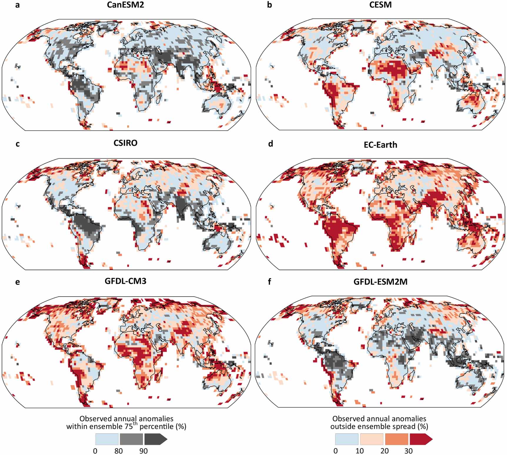
In figure 1, the results for the gridcell-based evaluation show that interannual variability over North and Central America, Europe and Western Russia is generally well captured by most models. The observational network in these areas is quite dense, which reduces the potential for observational uncertainty associated with this result. Generally, all models show a better representation of variability over the Northern compared to the Southern Hemisphere. Structural differences between models are apparent, in particular in tropical regions: while three SMILEs (CanESM2, CSIRO, and GFDL-ESM2M) show an overestimation of variability over South America, others show good agreement or an underestimation. Similar results are found in India, where CanESM2 and CSIRO overestimate the variability and other models do not (i.e. CESM, GFDL-CM3, GFDL-ESM2M). Overall, the evaluation highlights CESM and MPI (seen in figure 2(a)) as capturing precipitation variability most adequately over most parts of global land area. However, other SMILEs are equally good in some parts of the world and therefore interpretation depends on the region of interest.
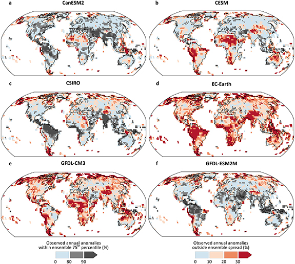
Figure 1. Evaluation of annual precipitation anomalies simulated by six different SMILEs compared to REGEN observed anomalies over land from 1955 until 2016. Light blue shading shows areas with a good representation of interannual precipitation variability. Grey shading suggests an overestimation of variability, red shading an underestimation of variability, and white areas show no-data. The grey shading shows the fraction of observed annual anomalies within the ensemble central 75th percentile range (e.g. for 85% of years the observational anomalies are within the ensemble 75th percentile range (light grey)). Red shading shows the fraction of observed annual anomalies outside the ensemble spread (e.g. for 25% of years the observed anomalies are outside the ensemble spread (above or below) (medium red shading)). Anomalies are relative to the climatological baseline of 1955–1974. Maps are cut to 60°S and 90°N.
Download figure:
Standard image High-resolution image
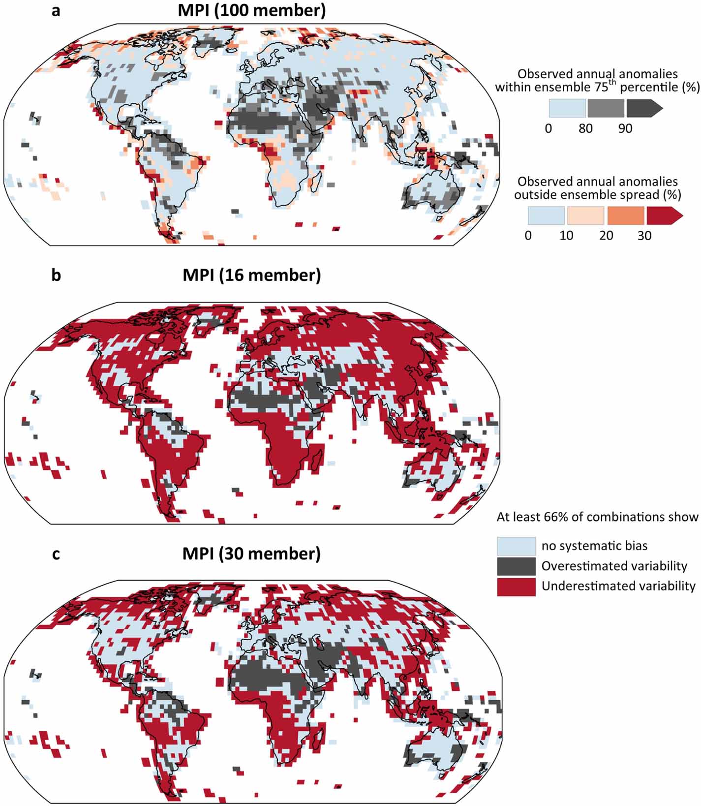
Figure 2. Evaluation of ensemble size dependence in interannual precipitation variability. (a) The evaluation result of the full MPI ensemble (100 member) following methods in figure 1. (b) Shows the result of 100 random combinations of 16 members drawn from the MPI ensemble. At least 66% of combinations show either (light blue) no systematic bias, (grey) overestimation of variability, or (red) underestimation of variability. The grey and red category are the generalization of the colorbars in panel (a). Grey represents at least 80% of observed annual anomalies within the ensemble 75th percentile range. Red represents at least 10% of anomalies outside the ensemble spread. (c) Shows the result of 100 random combinations of 30 members drawn from the MPI ensemble.
Download figure:
Standard image High-resolution imageWe checked whether the climatological baseline period for the anomaly calculation (figure S1 (available online at stacks.iop.org/ERL/16/084022/mmedia)) or the observational dataset (figure S2) itself affects the results. The general patterns seem to be unaffected by both, although individual gridcells might exhibit differences. Further, it was checked whether trends in interannual variability in the observations or SMILEs affects the results. We detrended both the observed and SMILE annual anomalies by applying a linear least-square fit to the data and subtracting it from the data. Over Africa and the northern High Latitudes, the detrended data shows a better representation, which might indicate a mismatch of a forced change in historical variability between some models and observations (figure S3). Although overall the general takeaways remain the same.
4.2. Influence of the ensemble size
The results in figure 1 might reveal an influence of the ensemble size on how adequately models can capture precipitation variability. The SMILEs with a small ensemble size (EC-Earth: 16, GFDL-CM3: 20) both show a tendency to underestimate variability across land, while the larger SMILE CanESM2 (50) tends to show an overestimation of variability. To analyze this further, we use an additional large SMILE, the 100 member MPI ensemble, to quantify the influence of the ensemble size on precipitation variability. We compare the full MPI ensemble (100 members) representing large ensemble sizes, with multiple random combinations of 16 and 30 members from the MPI, representing small and medium ensemble sizes.
An underestimation of precipitation variability over northern hemisphere mid- to high latitudes, as seen in the EC-Earth (figure 1(d)) and the MPI 16 members (figure 2(b)), are likely ensemble size dependent. Over the High Latitudes even ensemble sizes of 30 members might be too small (figures 1(c), (f) and 2(c)) and more members are needed. The SMILEs with at least 40 members (CanESM2, CESM, MPI) all seem to be better at representing High Latitude variability.
The underestimation of variability over South America, East Asia, South-East Asia, and Northern Australia, as seen in the ensembles with <30 members (figures 1(d), (e) and 2(b)), are partly ensemble size dependent. The under- or overestimation over the majority of Africa is rather related to structural uncertainty and not ensemble size, as well as over the Amazon, Northern Africa, the Middle East, and India.
5. Future changes in precipitation variability
Prior to the analysis of changes in precipitation variability, we have checked whether the six SMILEs are a good representation of the CMIP5 model suite, on different spectra of the rainfall distribution. For the change in mean precipitation, we can largely agree with previous studies (Lehner et al 2020, Maher et al 2021) on a good agreement of the SMILEs with CMIP5. The SMILEs project a global average change of 2.5% K−1 (figure S5(a)) which follows the early assumptions by Allen and Ingram (2002). Comparing the change in extreme precipitation with results for the CMIP5 ensemble (Pendergrass et al 2017), we can in addition assert this for extreme precipitation. The SMILEs project changes at a rate of 7.2% K−1 globally (figure S5(b)) in conjunction with the rate of near surface moisture change (O'Gorman and Schneider 2009).
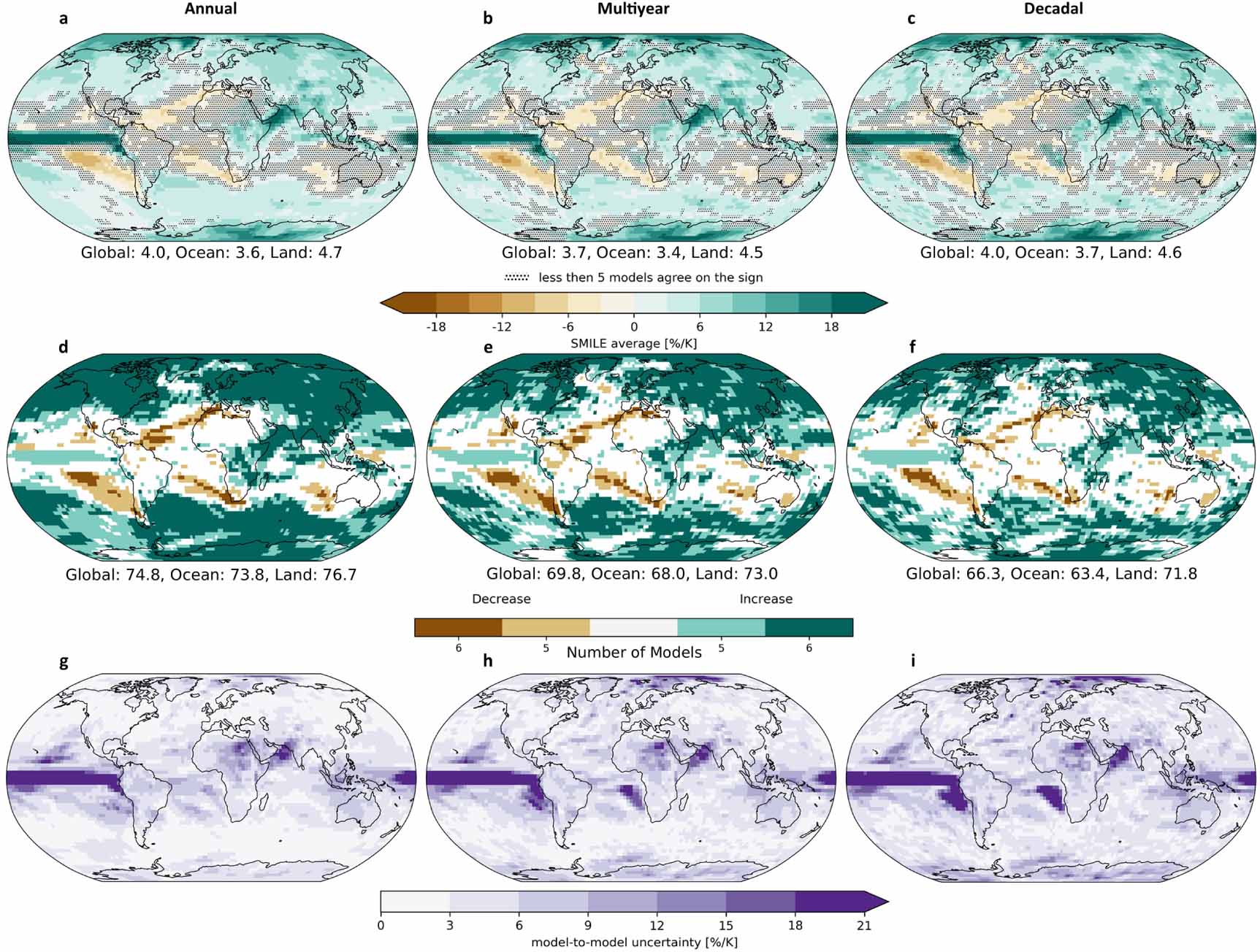
Precipitation variability increases globally by 3.7–4% K−1 for timescales of annual to decadal (figures 3(a)–(c)), which is higher than the increase in mean state precipitation (2.5% K−1, figure S5(a)) but lower than the scaling of near surface moisture change. Over land, where changes have the biggest impact on society, variability increases at a higher rate, around 4.5–4.7% K−1. Over oceans the increase is modestly lower, around 3.4–3.7% K−1. These scaling rates already show how remarkably similar the scaling rates are over all timescales. However, changes in interannual variability show higher model agreement over larger parts of the globe than for the longer timescales. Around 75% of gridcells globally show high model agreement for interannual variability changes, while only ∼66% of grid cells show agreement on decadal variability changes (figures 3(d)–(f)). Model agreement over land is slightly higher than over the ocean or globally.

Figure 3. Patterns of variability change by 2080–2099. Left column ((a), (d), (g)) shows maps for annual variability; center column ((b), (e), (f)) for multiyear variability; and right column ((c), (f), (i)) for decadal variability. Upper row (a)–(c) shows the multi SMILE forced response as the relative change scaled by the GMST change w.r.t. 1955–1974. Hatching indicates low model agreement (less than 5 models agree on the sign). Numbers below the panels indicate area weighted averages over the globe, ocean, and land in % K−1. Center row (d)–(f) shows the number of models agreeing on the sign of change (browns: negative/decreasing; greens: positive/increasing). White colors indicate low model agreement with less than 5 models in agreement. Numbers below the panels indicate the percentage of global, ocean, and land gridcells with model agreement. Bottom row (g)–(i) shows the model-to-model uncertainty in the forced response (standard-deviation across the individual SMILE's forced change).
Download figure:
Standard image High-resolution imageThe relatively large number of gridcells with high model agreement indicates that the individual SMILEs generally agree and show similar global rates. However, two distinctive exceptions must be mentioned. First, GFDL-ESM2M shows little to no change (0.1–0.8% K−1) in variability across all timescales (figures S6–S8). This could potentially be linked to a weakening of the ENSO amplitude and less frequent extreme El-Nino events as shown by the GFDL-ESM2M (Kohyama and Hartmann 2017). The GFDL-ESM2M has been shown to have a more realistic ENSO nonlinearity compared to other models from the CMIP5 archive. Kohyama and Hartmann (2017) argue for a La Nina-like warming rather than El Nino-like mean-state warming proposed by most other models. However, the causality of the proposed mechanisms needs to be further investigated as well as the connection to the here shown forced response of precipitation variability (or lack thereof) in the GFDL-ESM2M. Over the mid- and high latitudes, the GFDL-ESM2M is consistent with the other SMILEs, showing an increase in variability.
Secondly, EC-Earth shows globally considerably higher scaling rates for precipitation variability changes across all timescales, between 8.2 and 8.9% K−1 (figures S6–S8), which is above the near surface moisture change of 6–7% K−1. As shown in section 4, the EC-Earth shows smaller historical interannual variability, compared to other SMILEs, and generally underestimates historical variability. The small variability might be connected to small ensembles not being able to capture the full variance of modes of variability, as shown by Maher et al (2018) for ENSO variance. A smaller variability in the historical period can lead to higher percentage changes compared to a SMILE with a higher variability and the same absolute change. Both examples (GFDL-ESM2M and EC-Earth) show that model-to-model agreement on the sign might be given, but that structural uncertainty is still relevant for model-to-model agreement on the magnitude of change. These differences are highlighted by the model-to-model uncertainty (i.e. standard-deviation of the SMILE's forced changes) which are increasing from interannual to decadal timescales (figures 3(g)–(i)).
The areas with low model agreement in interannual variability and longer timescales over land (i.e. South America, Northern Africa, and Middle East) are consistent with the areas of high structural uncertainty shown in the previous section. Regions with low model agreement over the oceans are mainly around subtropical subsidence regions with decreasing precipitation variability (figures 3(a)–(c)) and decreasing mean state precipitation (figure S5(a)). Here, we find high model agreement in the centers, but declining model agreement towards the edges, due to differences in the geographic extent. We note that a point-wise comparison will conceptually underestimate the agreement of the models, as dynamical boundaries and features, such as the jet stream, or divergence and convergence zones are not geographically coincident between models (Madsen et al 2017, Brown et al 2020, Harvey et al 2020), despite possibly showing consistent trends within the features. For the subtropical descending regions, He and Li (2019) show that interannual variability is constrained by mean state precipitation and that the change in interannual variability is almost proportional to the change in mean state precipitation.
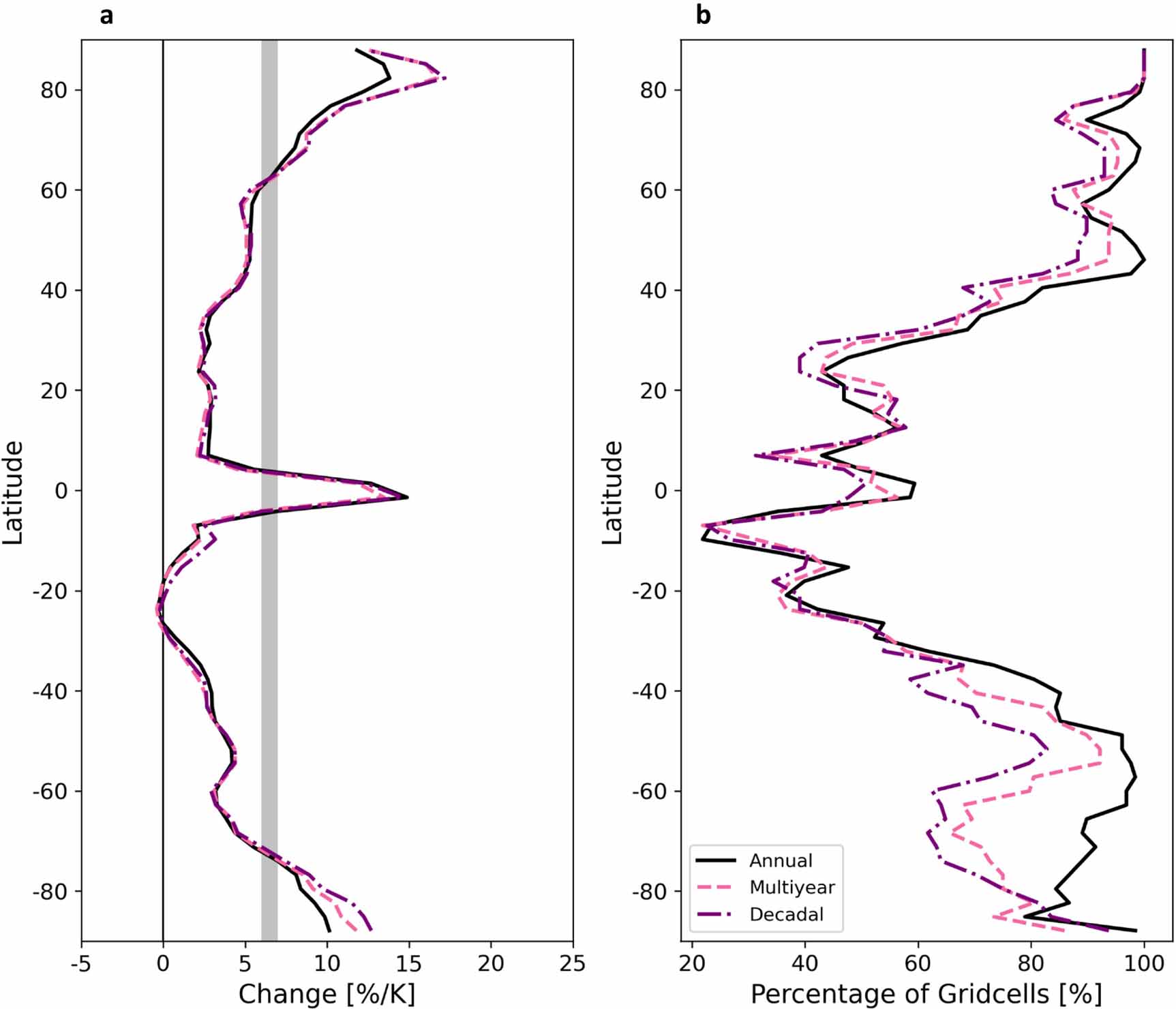
Regionally, precipitation variability strongly increases in all SMILEs over the Pacific ITCZ (figures 3(a)–(c)) across all timescales (except for GFDL-ESM2M), as also shown for mean and extreme precipitation (figures S5(a) and (b)). It needs to be noted that the model-to-model uncertainty is substantial over the ITCZ (figures 3(g)–(i)). However, the dynamical changes in the ITCZ are yet not well understood (Allan et al 2020). Precipitation variability increases over the South Pacific Convergence Zone (SPCZ) alongside a widespread increase in extreme precipitation. This might indicate that the change in precipitation variability is linked to an increase in severe weather events, which has been shown by Cai et al (2012) indicating a near doubling of zonal SPCZ event occurrence, although it needs to be acknowledged that climate-model simulations of the SPCZ still show persistent biases (Brown et al 2020 and references therein). In contrast, the south-eastern Pacific dry zone gets drier (figure S5(a)) and precipitation variability decreases, which aligns with the paradigm of wet-gets-wetter and dry-gets-drier found mostly over oceans. Generally, in the Tropics and Subtropics model agreement is much lower (<60% of gridcells) than in the mid- and high latitudes for all variability timescales (figure 4(b)).
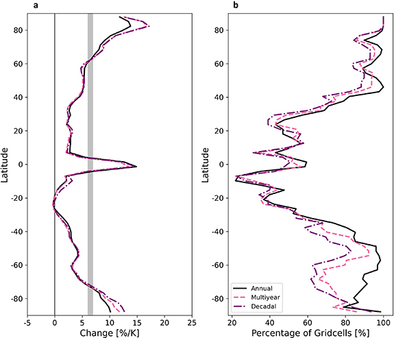
Figure 4. (a) Latitudinal zonal averages of precipitation variability change and (b) percentage of gridcells with high model agreement on the sign of change (at least 5 out 6 models agree) by 2080–2099. In panel (a) the vertical black line marks zero and the grey band indicates the Clausius-Clapeyron relation (6–7% K−1).
Download figure:
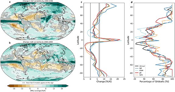
Standard image High-resolution imageOver the mid- and high latitudes, it is very likely that the hydrological cycle intensifies, and that variability increases across all timescales at scaling rates around or above the Clausius-Clapeyron (CC) relation of 7% K−1 (north of 60°N, figure 4(a)). The scaling rates are even higher for the change in wintertime variability (DJF) with 2xCC in the Arctic (figures 5(a) and (c)). An increase in arctic interannual precipitation variability was also shown by Bintanja et al (2020), linking the changes to an increased poleward moisture transport. Over North America, Dong et al (2018) link an increase in Mid-latitude wintertime variability to an increase in moisture (thermodynamical component), while the subtropical South is more dominated by a change in circulation variability (dynamical component). Over the northern hemisphere, at least 80% of gridcells show an increase in variability across all timescales. Over the southern hemisphere, interannual variability also shows high model agreement over at least 80% of gridcells, but longer durations show lower agreement over 60% and more of gridcells (figure 4(b)).
Figure 5. Forced changes in seasonal variability by 2080–2099. (a) Change in winter (DJF) variability; (b) change in summer (JJA) variability; (c) latitudinal zonal averages for annual and seasonal changes; (d) percentage of gridcells with agreement on the sign. In panel (c) the vertical black line marks zero and the grey band indicates the Clausius-Clapeyron relation (6–7% K−1).
Download figure:
Standard image High-resolution image
The SMILEs agree on an increase in variability across all timescales over the South Asian and East Asian Monsoon region which is consistent with Brown et al (2017a) for timescales shorter than decadal. Our results also indicate an increase in decadal variability in these regions. The increase in the South and East Asian Monsoon region is most noticeable in the change of the summertime variability (JJA) at rates above 7% K−1 (figure 5(b)).
Generally, the patterns for changes in precipitation variability are quite complex and on seasonal scales these patterns are even more complex, highlighting the importance of local dynamics boosting or attenuating changes.
6. Summary and conclusions
We have used six single-model initial-condition large ensembles (SMILEs) to analyze changes in mean and extreme precipitation, as well as precipitation variability across multiple timescales (annual to decadal) by the end of the century under the RCP8.5 emission scenario.
Mean and extreme precipitation increases in the multi-SMILE average at a rate of 2.5 and 7.2% K−1 globally following the theoretical scaling rates. These results indicate that the six SMILEs agree with the results from the CMIP5 models and are therefore a suitable super ensemble for mean state precipitation analysis, which recently has also been shown by Lehner et al (2020) and Maher et al (2021), and can now also be asserted to extreme precipitation.
We can show implicit evidence for a forced change in internal variability in a warming climate which leads to an increase in precipitation variability from interannual to decadal timescales. We can further show that the scaling rates are markedly stable across all timescales and that they can locally exceed the Clausius-Clapeyron relation (>7% K−1). Interannual precipitation variability increases at rates of 4% K−1 (4.7% K−1) globally (over land), multiyear variability increases at rates of 3.7% K−1 (4.5% K−1), and decadal variability at rates of 4% K−1 (4.6% K−1). Seasonal variability can exceed these rates especially over land in winter (DJF, 5.8% K−1) as well as locally, highlighting the importance of changes in local processes. These high scaling rates have considerable relevance for local climate adaptation plans.
The increase in precipitation variability implies an increase in precipitation volatility with an enhanced risk of swings between extreme dry and wet periods, as shown by Swain et al (2018) for California. This could pose challenges for communities that rely on precipitation as a primary water source. While projections remain uncertain over the majority of Africa, we can show an increase in precipitation variability over Eastern Africa across all timescales.
Over northern hemisphere mid- and high latitudes, model agreement on the sign is very high with at least 80% of gridcells showing an increase in variability across all timescales. Thus, while reducing model-to-model differences will only slightly improve model agreement on the sign, it will still improve agreement on the magnitude of change. Over the Tropics and Subtropics model agreement is considerably lower than elsewhere, which means that reducing structural uncertainty will improve both the agreement on the sign and the magnitude of change.
For interannual variability, the patterns from the SMILEs show considerable resemblance to results from the CMIP5 ensemble (Pendergrass et al 2017, He and Li 2019, Maher et al 2021), which shows that there is considerable amount of internal variability included in CMIP5. Further, it shows that the multi-SMILE ensemble can be a valuable tool to test the hypothesis derived from the CMIP5 ensemble, and extent our understanding of dynamical changes, such as ENSO, which drive local variability and could explain model differences (e.g. the lack of variability change in the GFDL-ESM2M).
Alongside the changes in precipitation variability, we conducted a first evaluation of historical interannual precipitation variability in the 6 SMILEs. While there are several caveats to consider (e.g. smoothing of precipitation variability during the interpolation and remapping process, temporal artifacts related to changes in the observational system, or varying degrees of quality of the underlying data) we mainly focused on the model-to-model differences rather than absolute biases. Overall, the evaluation highlights CESM and MPI as capturing interannual precipitation variability most adequately over most parts of global land area. The evaluation reveals that especially over the Tropics and Subtropics structural uncertainty remains critical, which is supported by the low model agreement on future forced changes in precipitation variability. Lastly, we show that small ensembles (less than 30 members) tend to underestimate historical annual precipitation variability (e.g. northern hemisphere mid- and high latitudes, Northern Australia, East Asia). This suggests that ensembles with at least 30 members are needed for a robust quantification of interannual variability of precipitation.
Acknowledgments
We acknowledge US CLIVAR for support of the Multi-Model Large Ensemble Archive (MMLEA). Data was analyzed using the Iris Python library (v2.4; https://scitools.org.uk/iris). R R W was supported by the ClimEx project, funded by the Bavarian Ministry for the Environment and Consumer protection. F L was supported by the Swiss National Science Foundation (Grant No. PZ00P2_174128). This work was partly supported by the Regional and Global Model Analysis (RGMA) component of the Earth and Environmental System Modeling Program of the U.S. Department of Energy's Office of Biological & Environmental Research (BER) via NSF IA 1844590, and by the National Center for Atmospheric Research, which is a major facility sponsored by the National Science Foundation (NSF) under cooperative Agreement No. 1947282. S S was supported by NASA award NNX17AI75G and by NSF's Southern Ocean Carbon and Climate Observations and Modeling (SOCCOM) Project under the NSF Award PLR-1425989, with additional support from NOAA and NASA.
Data availability statement
The GFDL-ESM2M daily data are publicly available through the Princeton Multi-ESM Large Ensemble Archive (http://poseidon.princeton.edu). All other SMILEs are available on the Multi-Model Large Ensemble Archive (MMLEA; www.cesm.ucar.edu/projects/community-projects/MMLEA/). The observational datasets are available on the FROGS database (Roca et al 2019) and are openly available at: https://doi.org/10.14768/06337394-73A9-407C-9997-0E380DAC5598.