

Abstract
According to the characteristics of forced and unforced components to climate change, sophisticated statistical models were used to fit and separate multiple scale variations in the global mean surface temperature (GMST) series. These include a combined model of the multiple linear regression and autoregressive integrated moving average models to separate the contribution of both the anthropogenic forcing (including anthropogenic factors (GHGs, aerosol, land use, Ozone, etc) and the natural forcing (volcanic eruption and solar activities)) from internal variability in the GMST change series since the last part of the 19th century (which explains about 91.6% of the total variances). The multiple scale changes (inter-annual variation, inter-decadal variation, and multi-decadal variation) are then assessed for their periodic features in the remaining residuals of the combined model (internal variability explains the rest 8.4% of the total variances) using the ensemble empirical mode decomposition method. Finally, the individual contributions of the anthropogenic factors are attributed using a partial least squares regression model.
Export citation and abstract BibTeX RIS

Original content from this work may be used under the terms of the Creative Commons Attribution 4.0 license. Any further distribution of this work must maintain attribution to the author(s) and the title of the work, journal citation and DOI.
1. Introduction
It is generally believed that long-term climate changes can be divided into two parts: the external forcing 'signals' (including both the anthropogenic and the natural forcing) and the internal variability (also called 'noise') of the climate system (Santer et al 2001, Hegerl et al 2007, Bindoff et al 2013). Of these, the longest-term and largest-scale climate changes are dominated by external forcing, with internal variability playing an essential role at the shorter term, smaller spatial scales. A good example is the recently heated discussion of global warming slowdown (Frankcombe et al 2015). Since the latter part of the last century, climate change attribution research has been based on the comparison of models and observations (Hasselmann 1993, Hegerl et al 1996, Tett et al 1999, Stott and Kettleborough 2002, Zhang et al 2006). An optimal fingerprint (OFP) is used to estimate the response coefficient of the climate change to external forcing. It can be implemented by generalized multiple regression (GMR), that is, observational climate changes are always regarded as the result of linear superposition of the climate change signals caused by external forcing, plus the internal variabilities of the climate system. Statistically, if effective radiative forcing and other impact factors are precisely quantified, their signals/responses can be near linearly reflected in the observational data. Thus there are a few studies on the causes of historical climate change based solely on using statistical methods to decompose climate change series into contributions of external forcing and internal variability (Haigh 2003, Staeger et al 2003, Lean and Rind 2008, Zhou and Tung 2013, Ribes et al 2017, Folland et al 2018).
The separation of the major components of climate change has always been one of the difficulties and is a core topic in modern climate change research. The simplest one is the linear detrending approach, where a linear trend is removed from the climate change series (Zhang and Wang 2013). The method is extremely simple and can be useful without any better estimates of forcing data (Frankcombe et al 2015), but has been shown to introduce biases in both amplitude and phase of the estimated internal variability (Mann and Emanuel 2006, Mann et al 2014). Another popular component extraction method is principal component analysis (PCA), or the similar statistical method termed empirical orthogonal functions in climatology (Preisendorfer 1988, von Storch and Zwiers 1999, Li et al 2020). The maximum remaining variance criterion used in PCA makes it a useful tool for information compression but also limits its ability for decomposing climate change into individual modes (Ilin and Valpola 2005). It can lead to problems like mixing different patterns in one extracted component (Kim and Wu 1999). The modified PCA method, which adopts orthogonal or oblique rotation of the PCs has proved to improve the interpretability of the extracted PCs (Richman 1986). An alternative rotational approach called independent component analysis (ICA), has also been applied to climate research since it was first proposed in about 2000 (Aires et al 2000, Hyvärinen et al 2001, Lotsch 2003). It is a statistical method for component extraction which can also be used for the rotation of PCs, and its basic assumption of the statistical independence of the extracted components can lead to more meaningful data representation (Richman 1986). More recently, Ilin et al (2006) developed a novel extension of ICA called denoising source separation framework, which does not necessarily exploit the independence assumption but uses means of temporal filtering or denoising procedure to look for interesting hidden components. MultiTaper method-singular value decomposition, a frequency-based SVD method, can be used to isolate and construct quasiperiodic or unstable oscillations that are spatially coherent but may exhibit phase-lags from site to site, which can be used to identify the most significant oscillations (Mann and Park 1999, Ribera et al 2020). Component extraction techniques also aid in identifying and interpreting the significant modes in climate change, such as pacific decadal oscillation (PDO) and Atlantic multi-decadal oscillation (AMO) (Hurrell 1995, Mantua et al 1997). For example, Folland et al (2018) successfully reconstructed the GMST series since 1891 from known natural and anthropogenic forcing factors, including internal climate variability, using a multiple regression technique. Additionally, Wu et al (2019) directly decomposed the contribution of long-term changes in global observed temperature into greenhouse gases (about 70%) and AMO and PDO (about 30%). Also Wei et al (2019) divided the de-trended global surface temperature sequence during the period 1850–2013 into three components: IAV, IDV and MDV showing that ENSO, PDO, and AMO each dominate the changes in these three components.
However, most of the above-mentioned statistical methods or models do not strictly distinguish the climate response of external forcing from internal variability. In addition, these models are also much less useful for detecting the individual contribution of each external forcing to climate change (especially for some highly related external forcings such as carbon dioxide and other greenhouse gases, etc). Due to the uncertainties in climate change observation, external forcing factor estimation and model simulation, it is very difficult to accurately quantify the contribution of external forcing to climate change. In addition, the traditional OFP analysis needs to carry out coupled model simulation experiments for attempts at distinguishing the contribution of different external forcings. At present, the latest Detection and Attribution Model Intercomparison Project (DAMIP) has only carried out relevant simulation experiments on fully-mixed greenhouse gases, CO2, anthropogenic aerosols, stratospheric-ozone, and natural forcings, but has not carried out systematic tests on other individual external forcing factors (Gillett et al 2016). The cost of carrying out such experiments is huge and cannot be borne by individuals or an independent research group alone. Therefore, there is still a wide space for further research on the methodology of the separation and relative contribution of climate change.
In this paper, based on statistical modeling experiments, we found that reasonable statistical models can be built to quantify the individual and total contributions of natural forcing, anthropogenic forcing (consisted of all components representing different human activities) and internal variabilities and successfully getting the contribution of these forecasting factors with known climate change time series and effective radiative forcing. Taking GMST series as the dependent variable, we set up a set of statistical models to separate the contributions of different forecasting factors and derive some interesting conclusions.
Thus the structure of this paper is arranged as follows: section 2 introduces the newly released China merged global surface temperature (CMST) dataset together with the radiative forcing data for anthropogenic and natural components used in this paper. In section 3 we set up a set of combined statistical models to model and separate the GMST changes into external forcing ('signals') and internal variabilities ('noise'), and also detect the individual contributions of human activities with a partial least squares regression (PLSR) model. Section 4 presents a brief summary and discussion of the paper.
2. Data and methods
2.1. GMST and radiation data
The station surface air temperature series have been quality controlled and homogenized (Xu et al 2018, Li et al 2021), and then converted to a 5° × 5° latitude and longitude grid dataset using the climate anomaly method (CAM) (Jones et al 1997), based on the 1961–1990 period. Then this China global land surface air temperature dataset (C-LSAT) was merged with NOAA's ERSSTv5 (Huang et al 2017), to develop a new CMST dataset and new GMST series, with 5%–95% uncertainty ranges evaluated (Yun et al 2019, Li et al 2020). The CMST dataset/series covers the monthly in situ data from January 1880 to December 2019. Comparative studies (Li et al 2020, 2021) showed that CMST has similar trends of global surface temperature and have similar uncertainties compared to other existing datasets. While the significant trends during the so called 'hiatus' period are identified by CMST, HadCRUTem4-Hybrid (infilled by the polar surface air temperature) (Cowtan and Way 2014) and ERA-5 (Simons et al 2017), etc.
Anthropogenic forcing data includes carbon dioxide (CO2), other greenhouse gases, atmospheric aerosols, snow albedo changes and land use (Hansen et al 2007, Myhre et al 2013, Shindell et al 2013), as well as the natural forcing data including volcanic eruptions and solar irradiation (Hegerl et al 2007, Bindoff et al 2013, Myhre et al 2013, Shindell et al 2013). Data for all these (best evaluation) were downloaded from Pangaea database and KNMI's Climate Explorer website (https://doi.pangaea.de/10.1594/PANGAEA.919662) (CMST), (C-LSAT2.0) and http://climexp.knmi.nl/selectindex.cgi?Id=someone@somewhere (radiative forcing), all downloaded in Jan 2020). The time range of these forcing data are from 1850 to 2017 as shown in figure S1 (supplement information (SI) (available online at stacks.iop.org/ERL/16/054057/mmedia)).
2.2. Models for separating the forced and unforced variations
Previous IPCC assessment reports stated that climate change signals can be decomposed into externally forced responses and internal climate (unforced) variability. Anthropogenic activities are becoming much clearer as the main contributors to surface air temperature warming, natural external forcing (such as volcanic eruptions, changes in solar output, represented by corresponding radiative forcing) also contribute to the climate change (Hegerl et al 2007, Bindoff et al 2013), and these contributions have also generally used a linear relationship expressed from at least one General Circulation Model through OPF method (Haywood et al 1997, Ramaswamy and Chen 1997). Therefore, a multiple linear regression (MLR) model is first used in this study, trying to separate the contribution of climate changes due to external forcing and internal variability.
Taking the GMST as the dependent variable, two variables (total anthropogenic forcing, natural forcing) are selected as the independent variables in the MLR model. We established the following MLR models of GMST change for the period 1880–2017:

where,  ,
,  are the total natural and anthropogenic forcing, respectively,
  is the residual series of the MLR model.
  are the regression coefficients evaluated by the ordinary least square (OLS) method. It should be noted that the recent OFP uses the total least square (TLS) method, which can be interpreted as the OLS with noise elimination (Bindoff et al
2013). However, in terms of linear regression in this paper, the OLS method will provide the best linear unbiased estimator (BLUE) of the regression coefficient according to the Gauss–Markov Theorem (Theil 1971), while the TLS needs more assumptions.
are the regression coefficients evaluated by the ordinary least square (OLS) method. It should be noted that the recent OFP uses the total least square (TLS) method, which can be interpreted as the OLS with noise elimination (Bindoff et al
2013). However, in terms of linear regression in this paper, the OLS method will provide the best linear unbiased estimator (BLUE) of the regression coefficient according to the Gauss–Markov Theorem (Theil 1971), while the TLS needs more assumptions.
Normally, if equation (1) is strictly a BLUE, its physical meaning is very clear, the MLR represents the part of the dependent variable (GMST) affected (caused) by the independent variables (the total natural and anthropogenic forcings), and  also represents internal variability in annual GMST. Since the residual analysis shows that there is no collinearity between natural forcing and artificial forcing, we only need to investigate if the residual has obvious negative or positive autocorrelation, which leads to the linear model no longer being BLUE, and the statistical significance of the variables is meaningless, that is, the simulation (fitting) of the model is invalid. In this case, equation (1) will need to be combined with ARIMA models (including the autoregressive (AR), moving average (MA), ARMA and ARIMA models, see Li (2020), and the supplemental information (SI)).
2.3. Multiple scales variations of internal climate (unforced) variability
Generally, the residual of a successful MLR model should have the following characteristics: (a) the residual obeys the normal distribution with zero mean; (b) the residual is a normal distribution with equal variances; (c) the residual sequence is independently distributed. That is, the residuals cannot be linearly fitted with new independent variables, leaving only periodic and random components. According to the MLR model, the residual represents the random error term of the model, which is the error between the fitted value and the actual value excluding the constant term in the independent variable interpretation space. In the sense of climate change, when the fitted external forced 'signal' is subtracted from the GMST anomaly series, the remaining series (i.e. the residual) can be considered to be mainly composed of the internal variability component ('noise' of climate change). We can know from the section 3 that the residual of MLR ('noise' or internal climate variability) still explains about 8.4% of the total variance of the GMST series. Due to the relatively more important contribution of internal climate variability has been claimed in the shorter term GMST variations in recent studies (Dai et al 2015, Frankcombe et al 2015, Folland et al 2018, Li et al 2020), we further decomposed the periodic signals in the residual series by an ensemble empirical mode decomposition (EEMD) method.
EMD model is a method of decomposing complex signals into a finite number of intrinsic mode functions (IMFs) through empirical mode decomposition:
where, imfi (t) is the ith IMF obtained by EMD; rn (t) is the signal residual component after n IMFs are decomposed and screened.
Each IMF component contains local characteristic signals of different time scales of the original signal. Compared with Fourier transform, wavelet decomposition and its basis function are derived from the data itself. Therefore, this method is intuitive, direct, posterior, and adaptive. EEMD is a noise-aided data analysis method based on the shortcomings of EMD method in modal aliasing (Huang and Wu 2008). The principle is that when a signal is added with a uniformly distributed white noise background, signal regions of different scales are automatically mapped to the appropriate scale related to the background white noise. Since the noise is different in each independent test, when the overall average of enough tests is used, the noise will be eliminated, and the only lasting and stable part is the signal itself (Huang et al 1998, Huang and Wu 2008, Wu et al 2011).
2.4. Separation of the individual external forcing's contribution
PLSR is an approach that is relatively new multivariate statistical data analysis tool. Because it can solve some problems that conventional ordinary multiple regression methods cannot, it has attracted the attention of researchers. PLSR provides a method for regression modeling of multiple dependent variables to multiple independent variables especially when there is a high degree of correlation among the variables tool, the analysis model is more reliable and the overall conclusion is most robust. It can also perform regression analysis, data structure simplification (PCA), and correlation analysis between two groups of variables (canonical correlation analysis) comprehensively. It is suitable for establishing regression models when there is a high degree of multiple correlation among the variables, which improves the deficiencies of traditional multiple regression analysis, making the analysis conclusions more reliable and robust. It is also suitable for regression modeling when the sample size is less than the number of variables (see the detailed introduction in text S2 in SI). In the past four decades, PLSR has been developed rapidly in both theory and practice, and its application field has also rapidly expanded to more social and natural science fields (Wang 1999, Li et al 2008). A PLSR model has also been used here to investigate the individual external forcings responses to the global and regional land precipitation variations like Li (2020).
3. The forced and unforced variations of GMST
3.1. The combined modeling of the external forcing responses
Taking the GMST as the dependent variable, two other variables (the total anthropogenic forcing and the natural forcing) are selected as the independent variables to construct the MLR model. We established the following combined model of MLR and ARIMA models of GMST variations for the periods of 1880–2017:
The analysis of the MLR model shows that neither of the above two variables (natural forcing  ; anthropogenic forcing
  ) can be eliminated (both are important). The adjusted square of the multiple correlation coefficient (total variance explained by the model) of the combined model is 91.6%; the analysis of variance shows that at the 5% level, the dependent variable and the two independent variables have a clear linear relationship, which proves the combined 'MLR and ARIMA' model is statistically meaningful (note that only the AR model is needed here); and both of the coefficients of the two independent variables (the anthropogenic and external natural forcing) have significant meaning. The variance inflation factors are 1.000, which also indicates that there is no co-linear relationship between the two independent variables; the Durbin–Watson (DW) test of the residuals also shows there is no first order autocorrelation in equation (3) (DW = 2.026, also see the table S1 of SI). From the above analysis and statistics, the combined model (3) are successful (BLUE) of GMST with the two independent variables, which also shows that the contribution of these two independent variables to the GMST variation is quite clear.
Figure 1(a) shows that the above regression fits well the GMST long term trend signals due to the response of the anthropogenic and natural forcing in the 138 years from 1880 to 2017. Figure 1(b) shows the residual of the combined model, and figure 1(c) shows the residual is a normal distribution with equal variances and the model is meaningful (BLUE) according to the three criteria mentioned in section 2.3. Of the two kinds of the external factors, the anthropogenic forcing has caused most of the GMST warming during the last 138 years. Before the second half of the 20th century, greenhouse gas emissions increased slowly, so the GMST also increased slowly, and it entered a period of rapid warming since the 1970s. However, we also notice that a certain contribution of the 'noise' (or internal variability), which explains about the rest 8.4% of the total variance contribution also agrees well with the previous studies (Li et al 2020). In addition, the fitted series was obviously affected by external forcing influences from five large volcanic eruptions: 1884 (Krakatau volcano, Indonesia, eruption in 1883), 1903 (Mt Pelee, Martinique, eruption in 1902), 1964 (Agung volcano, Indonesia, eruption in 1963), 1983 (Kilauea volcano, Hawaii USA, eruption in 1983), 1992 (Pinatubo volcano, Philippines, eruption in 1991) (Zhang and Zhang 1985, Hou and Li 2000).
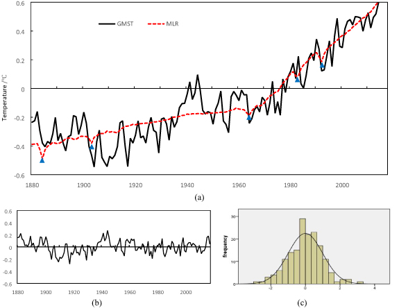
Figure 1. (a) The MLR fitting (red dashed line) of GMST anomalies (black solid line) change using anthropogenic and external forcing from 1880 to 2017 (the blue triangle indicates the year of the volcanos eruption); (b) the residual series of the MLR model and (c) its frequency distribution.
Download figure:
Standard image High-resolution image3.2. The multi-scales variations of internal climate (unforced) variability
Based on the EEMD model, the residual series of the above regression (figure 1(b)) is decomposed into six IMFs (the fluctuations at different timescales) and the remainder (figure 2). As can be seen from figure 2, there are obvious periodic signals in the internal variability of 2.9 years, 6.0 years, 13.8 years, 33.4 years, 69.8 years and 136.1 years. Among these, the first five IMF1–IMF5 (the variance contribution explained are 25.8%, 19.0%, 17.9%, 23.5% and 13.7%, respectively) passed the significant test at the 5% level, IMF6 explains only about 0.21% of the variance, and its periodicity was not significant. In other words, all these former five periodic changes are significantly reflected in the long-term variations of GMST. The further comparison also shows that the deposition of the multi-scale periodic signals is not sensitive to whether the external forcing effect is extracted in advance.
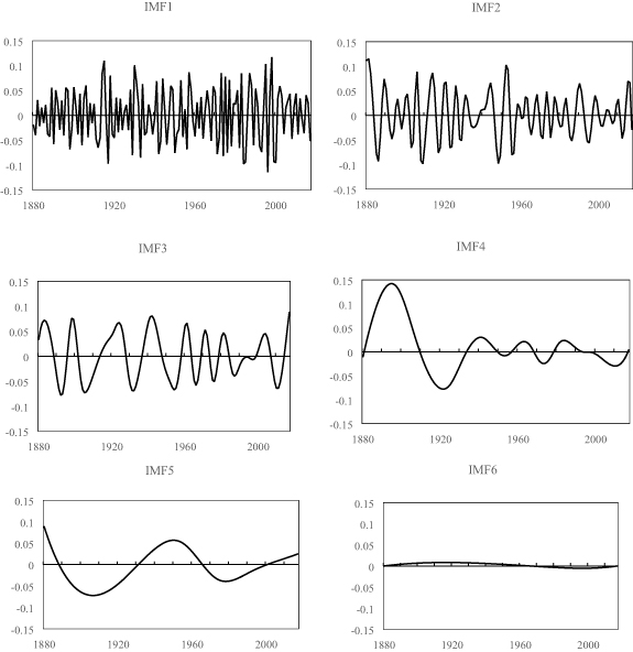
Figure 2. The EEMD results (IMFs 1–6) of internal variability from 1850 to 2017.
Download figure:
Standard image High-resolution imageFigures 2(a)–(f) also show that the internal climate variability term in the residual can be well decomposed into these several periodic signals. It can be seen that the inter-annual changes and the high and low phase of the GMST anomalies are well explained. IMF1, IMF2 explain the inter-annual variations (IAV) of the GMST, IMF3, IMF4 explain the IDV of the GMST, and IMF5 well explains the MDV warmer or colder fluctuation, and these five IMFs are exactly the eigenmodes with the largest contribution of variance, explaining a total of about 99% of the total variance of the combined model's residual, which in total accounts for about 8.4% of the total variance of GMST variations. Further, numerous previous studies indicated that the ENSO (2–7 year cycle), AMO (65–80 year cycle) and PDO/IPO (inter- decadal variation) are the dominant modulation signals of these three components (Dai et al 2015, Folland et al 2018, Wei et al 2019, Wu et al 2019). This agrees well with the multi-scales variations of internal climate (unforced) variability separated by EEMD in this paper.
3.3. Contribution of the individual external forcing response
Although the components of the natural and anthropogenic forcing responses have been separated through the above combined model of MLR and ARIMA, it is obviously not enough. More in-depth studies often need to clarify the contributions of individual forcing (such as CO2, aerosol, and even ozone in tropospheric and stratospheric layers), then the above models are no longer applicable. It has always been a difficult problem to separate the impacts of various anthropogenic forcings on climate change, that is, the 'confusion' between multiple independent variables. For example, the effects of urbanization and greenhouse gases on surface temperature variations are very similar (The average temperature increases, but the daily temperature range decreases). In terms of statistical language, these two variables may have a very clear correlation (Chong and Jun 2005) (this is very common in the case of multiple variables, namely multiple correlations or collinearity between factors, see table S2 in SI).
Figure 3 shows that the first six principal components (PCs) explained nearly 90% of the variance GMST, and it will not increase much with the introduction of more PCs. This shows the PLSR fits the GMST change well during the period of 1880–2017 with the first six PCs. Figure 3 presents the standardized PLSR coefficients of the independent variables. From figure 3 (and table S3 in SI), the coefficients for CO2, black carbon on snow (snow_BC), other GHGs, Aerosol and Natural forcing are significant at the 5% level, the land use's coefficient is marginally significant at 10% level, and the rest are insignificant. The independent variables including CO2, other GHG, land use and natural forcing, contribute to the GMST warming, while the rest (including aerosol, snow_BC, Ozone, water vapor and contrails (the last three variables' coefficients are insignificant)) contribute to cooling of the GMST. The slight difference with Myhre et al (2013) occurs in the warming (cooling) effect caused by the surface albedo change related to the land use and the black carbon on the snow surface. This shows there is still a large uncertainty about the correlation between surface albedo and global climate change currently (Schwaiger and Bird 2010, Sieber et al 2019).

Figure 3. (a) The PLSR principal components and the corresponding cumulative explanatory variance of dependent variables. (b) The standardized coefficient of the ten independent variables and the confidence interval under 95% confidence level.
Download figure:
Standard image High-resolution image4. Summary and discussion
Based on the current scientific understanding of the GMST change and its causes, this study developed a set of new statistical methods to quantify the contribution of external forcing to large-scale GMST change without relying on climate model simulations. This simplified model (figure 4) is based on the following assumptions: (a) it is assumed that the main external forcing factors affecting the process of climate change have been fully understood; (b) the impact of external forcing factors on climate change is linear and the contribution of different external forcing factors is additive. The following conclusions are achieved with the above approach:
- (a)When using the MLR to model the observed GMST change, the regression equation cannot satisfy the BLUE rules due to the autocorrelation and variance heterogeneity of the observed series, while the new model introduces an ARIMA model combined with MLR to solve this problem. Based on this, the human activities and natural forcing explain the main signals of GMST long term changes, which explain about 91.6% of the variance contribution;
- (b)The internal variability components of the GMST series can be further separated into obvious multi-scale periodic variation characteristics, which can be decomposed into three change components for IAV (3.9%), IDV (3.6%) and MDV (1.2%); showing that the contribution of the inner variability would be limited over the long term period, but it would be more significant during the shorter periods;
- (c)Taking into account the possible multicollinearity (correlation) between different external forcing factors, a PLSR is introduced to solve the problem of 'factor confusion' in this attribution study. PLSR model shows that the independent variables including CO2, other GHGs, land use and natural forcing, contribute to the GMST warming, while the rest including aerosol, snow_BC, water vapor, contrails and Ozone in stratosphere (the last four variables' coefficients are insignificant at 5% significance level) contribute to cooling of GMST. These conclusions are broadly consistent with the relatively complex detection and attribution results based on the comparisons between the observations and simulations (Hegerl et al 2007, Bindoff et al 2013), which also shows the 'robustness' of the above statistical methods.

Figure 4. The flow chart of the statistical deposition of the climate change.
Download figure:
Standard image High-resolution image
In addition, the whole process of the modeling is used to decompose and model the historical observation data. So in theory, it should also help to decompose the contribution of regional climate change caused by fully mixed radiative forcing factors, especially in the comparison of contributions to different regional climate changes; It is also helpful to separate the forced and unforced components of climate change of different lengths, and has the potential to provide a powerful and convenient supplement and reference for global and regional climate change attribution analysis.
However, at the same time, our study implies strict requirements on the 'purity' of the baseline observational dataset and the radiation forcing data. The uncertainties of both datasets will lead a certain uncertainties on the deposition results, which will be evaluated in depth with ensemble datasets (Sun et al 2021) in the future. The results described in this paper should be considered as preliminary since how to combine the simulation results of the climate system model to further conduct in-depth mechanism analysis of the statistical results is an important area for further research.
Acknowledgments
This study is supported by the National Key R&D Program of China (Grant Nos. 2018YFC1507705; 2017YFC1502301) and the Natural Science Foundation of China (Grant No. 41975105). The authors thank the editor and the anonymous reviewers for their constructive suggestions/comments in the initial reviews.
Data availability statement
The data that support the findings of this study are openly available at the following URL/DOI: https://doi.pangaea.de/10.1594/PANGAEA.919662.
Appendix
Table A1. List of acronyms (technical jargon).
| Acronym | Full name |
|---|---|
| MLR | Multiple linear regression |
| GMR | Generalized multiple regression |
| OLS/TLS | Ordinary/Total least square |
| BLUE | Best linear unbiased estimator |
| ANOVA | Analysis of variance |
| VIF | Variance inflation factors |
| DW test | Durbin–Watson test |
| ARIMA (AR, MA, ARMA) | Autoregressive integrated moving average (autoregressive, moving average, autoregressive moving average) |
| EEMD (EMD) | Ensemble empirical mode decomposition (empirical mode decomposition) |
| IMF | Intrinsic mode functions |
| PLSR | Partial least squares regression |
| PCA (PC) | Principal component analysis (principal component) |
| EOF | Empirical orthogonal functions |
| CCA | Canonical correlation analysis |
| IAV | Inter-annual variation |
| IDV | Inter-decadal variation |
| MDV | Multi-decadal variation |
| ICA | Independent component analysis |
| DSS | Denoising source separation |
| MTM-SVD (SVD) | MultiTaper method-singular value decomposition (singular value decomposition) |
| OFP | Optimal fingerprint |
Table A2. List of acronyms (climate).
| Acronym | Full name |
|---|---|
| C-LSAT | China-land surface air temperature |
| ERSST | Extended reconstruction sea surface temperature |
| CMST | China merged surface temperature |
| GMST | Global mean surface temperature |
| CAM | Climate anomaly method |
| PDO | Pacific decadal oscillation |
| AMO | Atlantic multi-decadal oscillation |
| ENSO | Elnino and southern oscillation |
| DAMIP | Detection and attribution model intercomparison project |
| DTR | Daily temperature range |
| OGHG (GHG) | Other greenhouse gases (greenhouse gases) |