

Abstract
Global mean surface temperature (GMST) shows considerable decadal variations superimposed on a pronounced warming trend, with rapid warming during 1920–1945 and 1977–2000 and warming hiatuses during 1946–1976 and 2001–2013. The prevailing view is that internally generated variations associated with the Interdecadal Pacific Oscillation (IPO) dominate decadal variations in GMST, while external forcing from greenhouse gases and anthropogenic aerosols dominate the long-term trend in GMST over the last hundred years. Here we show evidence from observations and climate models that external forcing largely governs decadal GMST variations in the historical record with internally generated variations playing a secondary role, except during those periods of IPO extremes. In particular, the warming hiatus during 1946–1976 started from a negative IPO but was later dominated by the eruption of Mount Agung in 1963, while the subsequent accelerated warming during 1977–2000 was due primarily to increased greenhouse gas forcing. The most recent warming hiatus apparent in observations occurred largely through cooling from a negative IPO extreme that overwhelmed the warming from external forcing. An important implication of this work is that when the phase of the IPO turns positive, as it did in 2014, the combination of external forcing and internal variability should lead to accelerated global warming. This accelerated warming appears to be underway, with record high GMST in 2014, 2015, and 2016.
Export citation and abstract BibTeX RIS

Original content from this work may be used under the terms of the Creative Commons Attribution 3.0 licence.
Any further distribution of this work must maintain attribution to the author(s) and the title of the work, journal citation and DOI.
1. Introduction
Global surface temperatures have experienced a significant long-term centennial time scale warming trend during the last hundred years (Trenberth et al 2007), owing to the effects of greenhouse gases (GHG) associated with the anthropogenic activities (e.g. Meehl et al 2005, Zhang 2016). In addition to GHGs, aerosols exert the second largest anthropogenic radiative forcing on the climate system (e.g. Mitchell et al 1995, Ming et al 2011), partially masking the GHG-induced warming trend. Superimposed on this long-term trend are periods of accelerated and reduced warming, the latter of which are often referred to as hiatus periods. Most notably between 2001 and 2013, warming largely stalled and global mean surface temperature (GMST) did not significantly increase (e.g. Easterling and Wehner 2009, Meehl et al 2011, Kosaka and Xie 2013, England et al 2014). Many studies have attempted to explain the recent global warming hiatus, often with a focus on the role of tropical Pacific sea surface temperatures (SSTs), as they have a large impact on global climate (Cane 1998). For example, the cooling in the eastern equatorial Pacific associated with the negative phase Interdecadal Pacific Oscillation (IPO) has been identified as a key component to the recent hiatus (Meehl et al 2011, Kosaka and Xie 2013, England et al 2014). Furthermore, since the tropical ocean basins are dynamically connected through the atmospheric Walker circulation, enhanced warming in the Atlantic (McGregor et al 2014, Li et al 2015) and Indian Ocean (Luo et al 2012) have been hypothesized to be a driver for the cooling in eastern Pacific during the recent warming hiatus.
The prevailing view is that the decadal GMST variations are dominated by internally generated variations associated with the IPO (Meehl et al 2013, 2016a, England et al 2014, Dai et al 2015, Trenberth 2015, Kosaka and Xie 2016, Fyfe et al 2016). The commonly used method in these studies is to add the IPO to externally forced variations to show an evolution consistent with observations. However, these studies neglect the potential contribution of external forcing on decadal GMST variations. For example, natural external forcing (Song and Yu 2015) including volcanic activity (Solomon et al 2011, Santer et al 2014) and solar radiation (Schmidt et al 2014, Soon et al 2015), and anthropogenic aerosols (Kaufmann et al 2011, Smith et al 2016), can also cause decadal variations in GMST. In addition, several studies from the early 2000s (Hegerl et al 1997, Tett et al 1999, Delworth and Knutson 2000, Stott et al 2000) reported that external forcing, both natural (solar irradiance and volcanic aerosols) and anthropogenic (GHG and sulphate aerosols), contributed to the long-term trend and decadal variations in GMST during the twentieth century. What role external forcing plays in the recent hiatus decade and its importance relative to the IPO remains an open question. Here we systematically explore the role of external forcing and internal variability in regulating decadal GMST variations based on newly available observations and Coupled Model Intercomparison Project Phase 5 (CMIP5) models. We find that externally forced variations dominate the observed GMST on decadal times scales during the past hundred years, though internally generated variations in eastern equatorial Pacific SSTs are also a significant driver of GMST, especially during extremes of the IPO.
2. Observations, model experiments, and method
Two monthly GMST products are used in this analysis: (1) NASA GISS Surface Temperature Analysis (GISTEMP, 2° latitude × 2° longitude, Hansen et al 2010); (2) Hadley Centre / Climatic Research Unit near surface temperature anomaly version 4 (HadCRUT, 5° latitude × 5° longitude, Morice et al 2012). Two monthly SST data sets are used: (1) Hadley Centre Global Sea Ice and Sea Surface Temperature (HadISST, 1° latitude × 1° longitude, Rayner et al 2003); (2) National Oceanic and Atmospheric Administration Extended Reconstructed SST version 4 (ERSST, 2° latitude × 2° longitude, Huang et al 2015, Karl et al 2015).
To distinguish the externally forced and internally generated variations, we use historical simulations before 2005 to which are appended Representative Concentration Pathway 4.5 (RCP4.5) runs for 2006–2013 from 18 CMIP5 models (ACCESS1-0, BNU-ESM, CCSM4, CESM1 CAM5, CNRM-CM5, CSIRO-Mk3-6-0, CanESM2, FGOALS-g2, GFDL-CM3, GISS-E2-H, GISS-E2-R, HadGEM2-ES, IPSL-CM5A-LR, MIROC5, MPI-ESM-LR, MRI-CGCM3, bcc-csm1-1, inmcm4). Note that using RCP4.5 experiments to extend the historical simulations is commonly used to bring historical runs up to the present (e.g. Kosaka and Xie 2013, Dai et al 2015, Takahashi and Watanabe 2016, Smith et al 2016). One realization of each simulation from these 18 models is used. The multi-model ensemble mean (MME) is defined as the arithmetic mean of models, with the same weight for each model. The twentieth century simulations are forced with observed atmospheric composition changes reflecting both natural and anthropogenic forcing (Zhou and Yu 2006, Jha et al 2014), so we assume the externally forced variations derived from the CMIP5 MME is representative of the effects of external forcing in observations assuming internally generated variations of the 18 CMIP5 models are averaged out (Dong et al 2014). This method was recently validated by Kosaka and Xie (2016), who demonstrated that the MME of historical simulations can capture the observed forced response quite accurately over the past 120 years. Therefore, we use the difference between the observed GMST (representing the combination of internally generated and externally forced variations) and the MME (taken as representing the externally forced variations) to estimate the internally generated variations. We assume that the externally forced and internally generated variations are additive; an assumption has been discussed by Taylor et al (2012) and Dong and Zhou (2014) and found to work reasonably well for most purposes. Note that CMIP5 models may be overly sensitive to greenhouse gas forcing and thus overestimate the warming trend relative to observations as suggested by the lack of agreement between satellite-observed and simulated radiative signatures in the tropics (e.g. Lindzen and Choi 2011, Dai et al 2015, Mauritsen and Stevens 2015, Bates 2016). Considering the range of climate sensitivities in CMIP5 models, using the ensemble mean of a large number of models to estimate external forcing on the climate system can reduce exposure to individual model biases. In addition, the pre-industrial control runs of 6 CMIP5 models are used to highlight the role of internally generated variations (table S1). The observed global average annual mean radiative forcing at the top of atmosphere (TOA) from CERES EBAF (Energy Balanced and Filled) (CERES EBAF-TOA Ed2.8, Loeb et al 2009) is compared with future projection scenarios of RCP2.6, RCP4.5, RCP6.0 and RCP8.5 from CMIP5 (Taylor et al 2012) in the discussion section to examine whether appending the RCP4.5 scenarios to historical runs is a reasonable way to characterize observed radiative forcing after 2006.
The effects of different external forcing factors are investigated by considering 129 specific forcing simulations from 8 CMIP5 models forced by historical all forcing (45 Hist. simulations), greenhouse gas (28 Hist. GHG simulations), natural factors (30 Hist. Nat simulations), and anthropogenic aerosol (26 Hist. AA simulations), as listed in table S2 (Taylor et al 2012). These 8 models are chosen for analysis as they offer the outputs of all the four types of specific forcing experiments. The relative contributions of GHG, AA, and natural (solar plus volcanic) forcing to the total externally forced GMST variations can be estimated by using the MME of each type of experiment.
To highlight variations on decadal timescales, a long-term linear trend is first removed, then an 8-year low-pass Lanczos filter (Hamming 1989) using 13 points is applied to the time series to remove inter-annual variations. The long-term linear trend is based on a least-squares linear fit to annual mean fields over the entire period of 1920–2013 for each region. For GMST, the trend over 1920–2013 is 0.63 °C per century for GISTEMP and 0.59 °C per century for HadCRUT. The purpose of removing the linear trend is to highlight the decadal variations rather than to completely remove externally forced signals, which can vary on decadal time scales. The 8-year low-pass filter is commonly used to remove inter-annual variations in previous studies (e.g. Han et al 2014, Dong et al 2016). We also examined the sensitivity of the results to different choices for low-pass window by using a 13-year low-pass filter (not shown), which indicates the robustness of our results. Note that the reduced effective degrees of freedom due to low-pass filtering has been taken into account when computing the confidence limits using a Monte Carlo technique (Dong et al 2014). To extract the leading decadal modes of global surface temperature, we performed an empirical orthogonal function (EOF) analysis of the decadal smoothed surface temperature datasets.
In our study, we consider the role of the IPO in affecting GMST. Some studies we cite discuss the role of the Pacific Decadal Oscillation (PDO) and others the IPO during global warming hiatuses and periods of accelerated warming. For the purpose of our study we consider these to be the same phenomena even though there are some distinctions (e.g. Newman et al 2016).
3. Results
3.1. Decadal variations in GMST and their relationship with regional SSTs
We start by noting the characteristics of decadal variations in GMST, which witnessed periods of rapid warming during 1920–1945 and 1977–2000 and periods of reduced or almost no warming during 1946–1976 and 2001–2013 (figures 1(a) and (b)). To explore the relationship between regional SST and GMST, we computed correlations on decadal timescales (figures 1(d) and (e)). For the tropical Indian Ocean, western Pacific Ocean and North Atlantic Ocean, observed decadal GMST variation shows a significant positive correlation with regional SSTs, while the eastern equatorial Pacific SST shows a weaker correlation with GMST. These results at face value do not support the prevailing view that IPO-related eastern equatorial Pacific SSTs dominate decadal variations of GMST (Dai et al 2015, Kosaka and Xie 2016). From this result we infer that the internally generated GMST variations associated with the IPO may be at times obscured by externally forced GMST variations.
Next the relative contributions of external forcing and internal variability are considered by examining the MME of CMIP5 historical plus RCP4.5 simulations, and pre-industrial control runs. GMST under external forcing reproduces the observed decadal variation reasonably well (figure 1(c)), with correlation coefficients between the CMIP5 MME and observations of 0.88 (HadCRUT) and 0.74 (GISTEMP) on decadal timescales (blue lines in figure 1), statistically significant at the 95% level of confidence. These results indicate the general dominance of external forcing in determining the decadal variations in the observed GMST. Results from specific forcing experiments from CMIP5 suggest that the decadal cooling during 1946–1976 mainly arose from naturally forced variations associated with the eruption of Mount Agung in 1963, though reduced growth in GHG concentrations during 1940s–1960s also made a secondary contribution (figure S1). The onset of this decadal cooling in 1946 also coincided with an IPO phase transition from positive to negative (Dai et al 2015), the contribution of which will be discussed further below. On the other hand, accelerated decadal warming during 1977–2000 mainly arose from the enhanced emission of GHGs, and secondarily from the reduced emission of aerosols after 1980s. The effect of volcanic aerosols from the eruptions of El Chichon in 1982 and Pinatubo in 1991 are clearly evident during this period. Correlation maps between SST and GMST indicates that external forcing drives consistent decadal variations of SST and GMST throughout the global oceans (figure 1(f)). However, it is noteworthy that while externally forced variations dominate the observed GMST on decadal timescales, it cannot account for the pattern of decadal variation in SSTs (cf. figures 1(g)–(i)). In particular, we observe that on decadal timescales, the tropical eastern Pacific, north Pacific and north Atlantic exhibit stronger magnitude variations than other basins (figures 1(g) and (h)), most likely due to internal variations associated with the IPO and AMO, respectively, since the pattern is not well reproduced by externally forced variations (figure 1(i)).

Figure 1 Time series (in °C) for annual GMST anomalies (red lines) and detrended 8-year low-pass filtered GMST (blue lines) from (a) HadCRUT, (b) GISTEMP and (c) external forcing from 18 CMIP5 models. Correlation coefficients between SST and GMST for detrended 8 year low-pass anomalies during 1920–2013 from (d) HadISST and HadCRUT, (e) ERSST and GISTEMP, and (f) external forcing. Stippling indicates regions exceeding the 95% statistical significance. Standard deviation of detrended 8-year low-pass filtered SST from (g) HadISST, (h) ERSST and (i) external forcing.
Download figure:
Standard image High-resolution imageConsidering internally generated variations alone based on pre-industrial control runs, the tropical Indian and Pacific Ocean SSTs show high correlation with decadal variations in GMST (figure S2). This IPO-like spatial pattern of correlation is robust in the 6 CMIP5 models. Also consistent across all the 6 models is the stronger magnitude in SST variations of the eastern equatorial Pacific relative to the Indian Ocean and western Pacific Ocean (figure S3). Dong et al (2016) also reported on the important role of internally generated variations associated with IPO in regulating decadal variations in Indian Ocean SSTs. Thus, combining the correlation maps (figure S2) with standard deviation maps (figure S3) we can infer that the eastern equatorial Pacific SST dominates GMST in the absence of significant external forcing, consistent with Kosaka and Xie's (2016) conclusion based on a series of pacemaker experiments with a global ocean-atmosphere coupled model.
3.2. Contributions of external forcing and internal variability to GMST and regional SSTs on decadal timescales
The relative contributions of external forcing and internal variability to decadal variations in GMST and regional SST are compared in figure 2. For GMST, the correlation coefficient between the observations and externally forced variations reaches 0.88 (figure 2(b)), statistically significant at the 95% level of confidence. These results clearly demonstrate that externally forced variations are the main contributor to the decadal GMST variations, accounting for about 77% of the observed variance. Internally generated variations also make a contribution (r = 0.56, significant at the 95% level of confidence), playing a secondary role in regulating decadal GMST during 1920–2013 (figure 2(c)). Regionally, both external forcing and internal variability contribute to decadal variations in Indian Ocean SST (figures 2(d)–(f)), consistent with previous studies (Han et al 2014, Dong et al 2016). Decadal variations in tropical western Pacific SSTs are largely influenced by external forcing, while eastern equatorial Pacific SSTs primarily reflect the dominance of internal variability (figures 2(g)–(l)). Both external forcing and internal variability are important for decadal variations of north Atlantic SSTs (figures 2(m)–(o)), confirming the findings in Booth et al (2012).
In particular, GMST and regional SST show a similar evolution on decadal timescales under the influence of external forcing (figures 2(b), (e), (h), (k), and (n)), consistent with the high correlation map between the two under external forcing (figure 1(f)). The 13 year running trend of externally forced GMST sharply peaks in the period 1991–2003 reflecting the rebound from Pinatubo induced volcanic aerosol cooling (Smith et al 2016). External forcing is still positive and high though during the recent hiatus decade even considering the effects of Pinatubo. A decadal cooling trend that occurs in association with the IPO phase transition from positive to negative phase in the late 1990s (figure 2(l)) leads to the GMST slowdown in the early 21st century as discussed in Kosaka and Xie (2013).
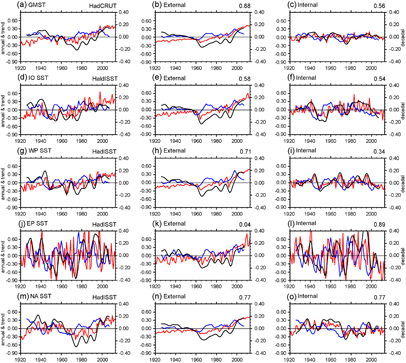
Figure 2 Time series for annual means (red; in °C), detrended 8 year low-pass filtered versions of the annual means (black; in °C) and the centered 13 year running trends of annual means (blue; in °C decade−1) for (a)–(c) GMST, (d)–(f) Indian Ocean SST (20°S–20°N, 40–120°E), (g)–(i) tropical western Pacific SST (20°S–20°N, 120–180°E), (j)–(l) eastern equatorial Pacific SST (10°S–10°N, 180°E-80°W), (m)–(o) North Atlantic SST (0–60°N, 70–180°W), shown as boxes in figure 1(d), from observations (HadCRUT and HadISST; left column), external forcing based on 18 CMIP5 models (middle column) and internal variability obtained from the difference between observation and externally forced variations (right column). The numbers at the top right denote the correlation coefficients between the observation and externally forced or internally generated variations on decadal timescales (black lines).
Download figure:
Standard image High-resolution image3.3. Dominant modes of externally forced and internally generated decadal variations in observed surface air temperature
The competing effects of external forcing and internal variability associated with eastern equatorial Pacific SSTs in determining the decadal evolution of GMST is a point we now elaborate on further. The first EOF mode (EOF1) of observed global surface temperature on decadal timescales shows warm anomalies in most regions except north Pacific (figures 3(a) and (c)). The global mean of this mode makes a positive contribution to GMST of 0.08 °C (GISTEMP) and 0.1 °C (HadCRUT) corresponding to one standard deviation change in the principal component (PC). In contrast, the second EOF in both the observations and in the externally forced response makes little contribution to GMST (figure S4).
EOF1 of externally forced surface temperature exhibits a warming pattern extending throughout the global oceans (figure 3 (e)). Albeit the pattern is different from the observations, PC1 of the forced response exhibits a similar overall evolution, its correlation reaching 0.75 with GISTEMP and 0.92 with HadCRUT (figures 3(b), (d), and (f))), which is statistically significant at the 95% level of confidence. These high correlations imply that decadal variations in GMST are strongly influenced by external forcing. However, comparing the EOF1 patterns between observations and externally forced variations reveals a large IPO-like difference in the Pacific, indicating that the IPO also contributes to GMST. Therefore, we suggest that external forcing and IPO-related SST in the eastern equatorial Pacific, which is dominated by internal variability, are the two key factors in affecting the decadal variations of GMST.

Figure 3 The leading EOF pattern (in °C) and associated standardized principal component (PC) of global surface air temperature based on 8 year low-pass filtered annual anomalies after the long-term trend for 1920–2013 is removed from (a), (b) GISTEMP, (c), (d) HadCRUT and (e), (f) external forcing based on 18 CMIP5 models. Values shown the top-right of the left panels represent the percentage variance explained by each mode, and those of the right panels represent the correlation coefficient with PC1 of external forcing. Values shown on in the middle of the left panels represent the GMST anomalies corresponding to one standard deviation of each PC.
Download figure:
Standard image High-resolution imageWe further conducted EOF analysis on pre-industrial control runs from CMIP5 models to investigate the dominant modes of internally generated decadal variations in global surface temperature. Common to all the 6 CMIP5 models, a robust IPO-like pattern emerges as the dominant mode of the decadal surface temperature variations, with a positive contribution to GMST (figures S5 and S6). However, the magnitude of IPO-like influence on GMST is much weaker than that of externally forced variations, ranging from 0 to 0.05 °C, which corresponds to one standard deviation in PC1 based on 6 CMIP5 models (figures S5 and S6). This is not surprising, given the non-uniform spatial pattern of IPO-like mode. Therefore, we infer that internally generated variations can overwhelm externally forced variations in GMST only when IPO-related SST in the eastern equatorial Pacific is unusually strong.
To roughly estimate the contribution of the eastern equatorial Pacific on decadal variations in GMST, we regress decadal variations in eastern equatorial Pacific SST on surface air temperature (figure S7). The regression pattern is very similar to that of the IPO. This pattern makes a positive contribution to GMST of 0.06 °C (for HadCRUT and GISTEMP) associated with one standard deviation in eastern equatorial Pacific SST on decadal timescales (figure S7). Therefore, warming of eastern equatorial Pacific contributes to an accelerated warming in GMST, while the cooling during the first decade of the 21st century would lead to a reduction in GMST, consistent with previous studies (e.g. Dai et al 2015, Kosaka and Xie 2013, 2016).
Thoma et al (2015) and Meehl et al (2016b) predicted a shift in the phase of the IPO from negative to positive around 2013–15 and thus an end to the global warming hiatus that began in 2000. In addition, Meehl et al (2016b) predicted a resumption of accelerated global warming over 2013–2022 and Thoma et al (2015) over 2016–2024 from the combined effects of external forcing and a warm phase of the IPO. Indeed, a shift in the phase of the IPO has occurred (www.ncdc.noaa.gov/teleconnections/pdo/) coincident with the development of El Niño conditions in 2014–16 (McPhaden 2015) and it appears that accelerated warming is underway, with GMST reaching three successive record highs in 2014, 2015 and 2016 (Trenberth 2015, Fyfe et al 2016, Yan et al 2016, www.cnn.com/2017/01/18/world/2016-hottest-year/index.html).
3.4. Factors influencing GMST during periods of rapid warming and warming hiatuses since 1920
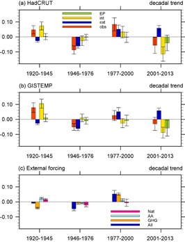
To quantify the relative importance of different external forcing factors and internal variability mainly from eastern Pacific SST in generating decadal variations in GMST, we examine the MME of CMIP5 models, focusing on the four distinct decadal periods suggested by the observations (figure 4 ). Note that the externally forced variations from the MME of 45 historical simulations based on 8 CMIP5 models (table S2; blue bars in figure 4(c)) are in good agreement with the 18 CMIP5 models (blue bars in figures 4(a) and (b)). Decadal time scale linear trends during each period are derived after removing the long-term centennial time scale linear trend over 1920–2013 for each product. Decadal warming during 1920–1945 and 1977–2000 and decadal cooling during 1946–1976 and 2001–2013 are consistent in the two products (red bars) with the decadal cooling during 2001–2013 reflecting the recent global warming hiatus. Though GHG forcing dominates the long-term warming trend in GMST during the last hundred years (e.g. Meehl et al 2005, Zhang 2016), it exhibits significant decadal variations, with weaker magnitudes than the long term centennial trend during 1920–1945 and 1946–1976 and stronger afterwards (figure 4(c)).
Figure 4 Decadal trends in GMST after removing the long term linear trend over 1920–2013 (in °C decade−1) during the periods 1920–1945, 1946–1976, 1977–2000 and 2001–2013. (a) Values derived using HadCRUT, with the full observed trends in red, the externally forced trends (obtained from the MME of 18 CMIP5 models) in blue, the values of the internally generated variations (based on the difference between HadCRUT and MME) in yellow, and the values contributed by the equatorial eastern Pacific SSTs in green. (b) As in (a), but using GISTEMP. (c) The corresponding externally forced decadal trends, and their components, as given by the 8 CMIP5 models of table S2; full trends from external forcing in blue, GHG components in orange, AA components in light blue, naturally forced components in pink. The error bars denote the 95% confidence limits for the linear trends. Note: in figure 4(c), results are given only for the first three decadal periods, since the components of the historical forcings are not available for the full period 2001–2013 (see text for further detail).
Download figure:
Standard image High-resolution image
The warming hiatus during 1946–1976 coincided with a cold phase of the IPO in observations (figures S7(a) and (b)), for which we would expect internally generated SST variations from the eastern equatorial Pacific to play a role (England et al 2014, Dai et al 2015). However, based on CMIP5 models, externally forced variations, mainly from the eruption of Mount Agung in 1963, significantly contributed to the global warming hiatus during 1946–1976 as well (pink bar in figure 4(c); see also figure S1), while internally generated variations show a small contribution only for HadCRUT (figure 4(a)). The reason that internal variations appear to play only small role during 1946–1976 may be that the IPO was in cold phase at this time, but there were no significant trends in its time series over this period (figures S7(a) and (b)). Time evolution of 13-year running trend in GMST after the long-term linear trend is removed exhibits negative decadal trends during 1946–1976 (black lines in figure S8(a)). This result indicates that internally generated variations from the IPO dominated decadal cooling at the beginning of this period (red lines in figure S8(a)) with weaker magnitude than the observed GMST cooling. Later, naturally forced variations due to volcanism in 1963 had major impact (Zhang 2016) along with a weaker impact from reduced growth in GHG concentrations before 1960 based on CMIP5 models (figure S8(b)). Therefore, the change in the IPO to a negative phase in 1946 started the decadal cooling, which was subsequently further accelerated by the eruption of Mount Agung in 1963. As a result, both internally generated and externally forced variations induced the warming hiatus during 1946–1976, confirming the statement in Zhang (2016) that stressed the role of IPO during 1940s–1950s and the importance of volcanic forcing during 1950s–1960s.
We attribute the decadal warming during 1977–2000 to externally forced variations, driven primarily by the enhanced increase in GHG emissions (orange bar in figure 4(c)). Warming due to the eastern equatorial Pacific SSTs in the late 1970s may have played a role in both ending the warming hiatus during 1946–1976 and contributing to the accelerated warming in 1977–2000 (figure S8(a)). Indeed, England et al (2014) and Dai et al (2015) have suggested that the accelerated warming during 1977–2000 was IPO driven.
For the recent global warming hiatus during 2001–2013, the cooling effect from internal variability (yellow bars) overwhelms the warming effect of external forcing (figures 4(a) and (b)). The effect of eastern equatorial Pacific SST accounts for much of the cooling from internal variability (green bars), though for HadCRUT its contribution is significantly smaller than the total of internally generated variations. The positive AMO phase (Liu 2012, McGregor et al 2014, Li et al 2015) and the uncertainty of the regression estimates (figure S7) may account for this difference. To quantitatively isolate the contribution of eastern equatorial Pacific SST, dynamic-model-based attribution studies have a distinct advantage (Dong et al 2016) and are needed for further study. Nevertheless, the results confirm those of Kosaka and Xie (2013) in that the cooling of eastern equatorial Pacific SST led to the recent hiatus in global warming. However, the eastern equatorial Pacific SST variations cannot account for the internally generated variation in decadal warming during 1920–1945 (figures 4 and S8(a)). The early twentieth century is a period for which we lack adequate observational coverage to accurately define GMST trends (Deser et al 2010, IPCC 2013) and for which we are less confident in the CMIP5 models' representation of those trends (IPCC 2013).
4. Summary and Discussion
The main motivation of the present study is to explore the relative importance of external forcing and internal variability in regulating GMST on decadal timescales and to clarify the relationship between GMST and regional SSTs. We have analyzed observed surface temperature datasets and a wide variety of CMIP5 coupled climate models to systematically quantify the relative contribution of externally forced and internally generated variations during 1920–2013. Our main conclusions are that:
- Superimposed on a pronounced long-term centennial time scale linear warming trend during the last hundred years due to GHG forcing, GMST also shows considerable decadal variations. These include rapid warming during 1920–1945 and 1977–2000 and periods of reduced or no warming during 1946–1976 and 2001–2013
- Decadal variability in observed GMST is dominated by externally forced variations due to GHGs, aerosols and volcanic forcing, while internally generated variations in general play a secondary role. At times internal variability can dominate GMST, especially during periods of IPO extremes. Though the IPO may be modulated by external forcing to some extent (Dong et al 2014, Smith et al 2016), it is fundamentally a mode of internal natural variability that accounts for about 80% of the decadal variations in the eastern equatorial Pacific SST (figure 2(l)), the key region of IPO.
- Decadal variations in observed GMST are well correlated with decadal SST variations in the tropical Indian Ocean, western Pacific Ocean and North Atlantic Ocean, suggesting that these regions are strongly influenced by external forcing. Conversely, decadal variations in observed GMST are less well correlated with eastern equatorial Pacific SSTs, where internally generated variations related to the IPO are prominent.
- The global warming hiatus during 1946–1976 mainly started from the onset of a cool negative phase IPO, but the volcanic eruption of Mount Agung in 1963 eventually played a dominant role, with reduced growth in GHG concentrations making as secondary contribution. The subsequent accelerated warming during 1977–2000 was primarily due to increased GHGs emissions. However, warming due to the IPO phase transition in the late 1970s contributed to the accelerated warming in 1977–2000 and to ending the warming hiatus of 1946–1976. In contrast, the contribution of cooling from internal variability overwhelmed the warming from external forcing during the most recent hiatus that began around the turn of the 21st century when SSTs in the eastern equatorial Pacific exhibited a strong cooling. With the onset of a positive phase of the IPO in 2014, an acceleration in global warming has occurred, with consecutive years of record high GMST in 2014, 2015, and 2016.
The relationship between the El Niño–Southern Oscillation (ENSO) and GMST on interannual time scales has been broadly reported in previous studies (e.g. Mann and Park 1994, Yulaeva and Wallace 1994, Klein et al 1999). In particular, during El Niño the ocean loses heat to the atmosphere, which elevates GMST, while during La Niña the ocean gains heat from the atmosphere causing GMST to cool. The IPO can be interpreted in part as the low frequency (inter-decadal) envelope of higher frequency ENSO variations (Zhang et al 1997). Thus, periods of positive IPO (decades dominated by El Niños) lead to warm GMST anomalies, while periods of negative IPO (decades dominated by La Niñas) lead to cold GMST anomalies. Thus, the interpretation of the role of the IPO in GMST inextricably involves consideration of the ENSO cycle.
In this study, we use RCP4.5 runs from CMIP5 to extend external forcing beyond 2006. To examine the reliability of this procedure, which is commonly used by other investigators (see section 2), we compare the observed radiative forcing with different RCP scenarios for 2005–2015 (figure S9). All four RCP scenarios share a synchronous evolution in radiative forcing, with stronger magnitudes than the observed 1.3 Wm−2 increase in TOA radiative forcing. Previous studies estimated that increasing GHGs have led to an increasing TOA radiative imbalance of order 0–1 W m−2 since 2000 (Trenberth 2009, Trenberth and Fasullo 2013). Allan et al (2014) reconstructed the increase as 0.62 ± 0.43 Wm−2 based on satellite data, atmospheric reanalyses and climate model simulations for 2000–2012 period. The overestimates from CMIP5 RCP scenarios may be because they only consider the effects of external forcing, while observations reflect the combination of both externally forced and internally generated variations. Though the results presented here are insensitive to the choices of which RCP scenarios are used after 2006, if we use the observed TOA forcing rather than RCP forcing, the positive contribution of external forcing would be weaker and the resultant negative effect of internal variability derived from the difference between observation and externally forced variations would also be weaker. However, we would still conclude that internal variability dominates the recent global warming hiatus. A more detailed analysis of the TOA radiative forcing during most recent decade needs further study.
Acknowledgments
This research was performed while the first author held a National Research Council Research Associateship Award at NOAA/PMEL. The data used are listed in the references, and the outputs from CMIP5 models can be downloaded at www.ipcc-data.org/sim/gcm_monthly/AR5/Reference-Archive.html. This is PMEL contribution no. 4536.