

Abstract
While Arctic sea ice is changing, new observation methods are developed and process understanding improves, whereas gaps in observations and understanding evolve. Some previous gaps are filled, while others remain, or come up new. Knowing about the status of observation and knowledge gaps is important for interpreting observation and research results, interpretation and use of key climate indicators, and for research and observation planning. This paper deals with identifying some of the important current gaps connected to Arctic sea ice and related climate indicators, including their role and functions in the sea ice and climate systems. Subtopics that are discussed here include Arctic sea-ice extent, concentration, and thickness, sea-ice thermodynamics, age and dynamic processes, and biological implications of changing sea ice. Among crucial gaps are few in situ observations during the winter season, limited observational data on snow and ice thickness from the Arctic Basin, and wide gaps in biological rate measurements in or under sea ice. There is a need to develop or improve analyzes and products of remote sensing, especially for new sensors and technology such as remotely operated vehicles. Potential gaps in observations are inevitably associated with interruptions in long-term observational time series due to sensor failure or cuts in observation programmes.
Export citation and abstract BibTeX RIS

Original content from this work may be used under the terms of the Creative Commons Attribution 3.0 licence. Any further distribution of this work must maintain attribution to the author(s) and the title of the work, journal citation and DOI.
1. Introduction and background
The identification of gaps in understanding the roles and functions of Arctic sea ice is important for assessing data and new findings of Arctic sea ice changes, and to develop research and monitoring strategies. The goal of this paper is to summarize and detail important current gaps of knowledge, and observation gaps related to Arctic sea ice, and, to a limited extent, to discuss the recent development of detecting gaps and ways and strategies for filling them. The paper includes discussing gaps in connection with key sea ice climate indicators.
On the first view, it might be easier to detect observation gaps rather than knowledge gaps. But the two things go hand in hand; more knowledge, i.e. an improved understanding of the system is also necessary to make better decisions on where to do which type of observations.
Our discussion of gaps is not comprehensive. Sea ice is a broad and interdisciplinary scientific subject with numerous sub-disciplines and processes at play, and we by no means claim to present here a complete overview on Arctic sea ice gaps, rather a selection of some of the important ones. Our focus is on the observational record and methods used to observe a variety of sea ice conditions.
The starting point for this work is based on the sea ice chapter of the recent Arctic Marine Assessment Program (AMAP) Snow, Water, Ice and Permafrost Assessment (SWIPA) 2017 report (AMAP 2017), where knowledge and observation gaps were addressed regarding (i) sea-ice extent, concentration, and thickness, (ii) sea-ice thermodynamics, age and dynamic processes, and (iii) biological implications of changing sea ice, respectively (Barber et al 2017). Of those topics, especially ice extent, thickness and age are often used as indicators of climate change, which makes existence or potential existence of gaps even more relevant to be discussed.
Gaps that are addressed in the SWIPA 2017 report are, for example, the fact that there are very few in situ observations in winter; limited data available on snow thickness from the Arctic Basin; and that there is the need to develop or improve analyzes and products of remote sensing, including for example new sensors or satellites.
How have the gaps discussed here changed over time? On one hand, the number of gaps is gradually becoming less since some scientific questions are answered or observation systems put in place. On the other hand, more sophisticated methods and models may also need better input data, which do not always exist, and they might identify new processes for consideration, meaning that new gaps will arise. Changes in Arctic sea ice can lead to new or different sea ice processes becoming dominant, which may lead to new knowledge requirements, and by extension new methods that will need to be tested and validated.
Information on how gaps have changed over time will be supported by comparing statements and subchapters on knowledge gaps from the SWIPA 2017 report (AMAP 2017) and recent literature with statements in ACIA (2005), SWIPA 2011 (AMAP 2011) and other earlier assessments.
Uncertainties of observational methods are not explicitly gaps of knowledge, but they can affect our ability to gain new insights on processes of interest. For example, if a method is too coarse to reveal heterogeneity at some spatial scales, it is difficult to assess the role of that heterogeneity on relevant processes. Therefore, we also include to some extent uncertainties in the discussion. Under uncertainties we understand the sum of several contributions: (i) the difference between a true quantity and its observed value—bias or accuracy; (ii) the repeatability with which a quantity is observed by the same method—precision; (iii) the degree with which the spatiotemporal distribution of a quantity is observed by the same method—representativity error; and (iv) the degree with which the spatiotemporal distribution of a quantity is observed by the same method with unchanged contributions (i)–(iii)—stability. When discussing the uncertainties of different methods, reasons for uncertainties are often related to the physics of sensors, assumptions/simplifications of the methods, the sea ice system, or economic limits. While some uncertainties can be reduced through ideas and action, others cannot be changed. Methods that have low accuracy or coarse spatial or temporal resolution often have other advantages that makes them attractive for applications where the accuracy is not the one and only criterion for the usability/usefulness of the method but the high stability is more relevant.
Although we focus here on gaps related to Arctic sea ice, several of the points raised apply equally for Antarctic sea ice, especially in recent years as the Arctic sea ice has transitioned to a state with a larger portion of seasonal sea ice at the cost of older, multiyear ice.
2. Existing gaps and uncertainties
2.1. Gaps in knowledge for sea ice concentration, extent and thickness
The sea ice concentration and extent record from passive microwave instruments provides a nearly complete and consistent record since late 1978. On one hand, this almost 40 year long time series is a very important tool for climate studies, and it is used widely as a climate indicator to quantify and illustrate Arctic sea ice change. On the other hand, the fact that the time series is limited to four decades, that it has limited spatial resolution, some varying data quality, and uncertainty depending on season and changing satellite sensors over time all limit the applicability of the time series. Intercalibration between sensors has not always been optimal (Eisenman et al 2014). This could be improved via use of longer overlaps period that are now available, employing better calibrated source data and, as is now being done in some products (Comiso et al 2017, Lavergne et al 2019), implementing adaptive time-varying algorithm coefficients that adjust for changing surface conditions. Nevertheless, there is a looming gap due to the potential loss of satellite coverage. Passive microwave sensors have been routinely launched since 1987 and for many years multiple sensors have been in orbit. However, recent failures have reduced the number currently operating sensors and have significantly increased the risk of a gap in coverage in the next years. AMSR-E failed in 2011, and the DMSP F-19 SSMIS failed in early 2016 after only two years of operation. In April 2016, the F-17 SSMIS started behaving anomalously and its data quality has been reduced. The suite of DMSP SSMI/SSMIS instruments has been the workhorse of passive microwave observations, but all currently operating (as of June 2018) SSMIS instruments (F-16, F-17, F-18) have been in orbit for at least 8.5 years, well beyond their design lifetime of three years (figure 1). The JAXA AMSR2 sensor, operating for a little over six years (as of June 2018) is the youngest passive microwave sensor, but it is now also past its design lifetime (five years). The only remaining sensor potentially ready to be launched in the near future (the DMSP F-20 SSMIS) has been cancelled.

Figure 1. Current and future polar orbiting passive microwave coverage. Acronyms used in figure: AMSR: Advanced Microwave Scanning Radiometer; CMA: Chinese Meteorological Adminitration; DMSP: Defense Meteorological Satellite Program (U.S. Department of Defense); EUMETSAT: European organization for the exploitation of Meteorological satellites; ESA: European Space Agency; JAXA: Japanese Aerospace eXploration Agency; MetOp: Meteorological operational satellite; SSMIS: Special Sensor Microwave Imager and Sounder; WSF: Weather Satellite Follow-on (DoD).
Download figure:
Standard image High-resolution imageWhile discussions concerning follow-on sensors are ongoing (including an AMSR follow-on, a EUMETSAT instrument on their METOP constellation, and possible new US radiometers) these are all likely to be a minimum of five years from launch. At that point, the youngest sensor commonly used for climate monitoring (AMSR2), if still operating, would be nine years old. There is a passive microwave sensor (MWRI) on the Chinese FengYung-3B and -3C platforms. This has not been employed as part of the long-term passive microwave sea ice climate record, but has potential to fill the looming gap due to the loss of current capabilities. First intercalibration efforts of the FY-3C satellite data with other passive microwave satellite data have been made (Li et al 2016, Wang et al 2018, Wu and Liu 2018).
Another important, but more difficult to measure sea ice climate indicator is sea ice thickness. Significant development has been made to quantify sea-ice thickness and its seasonal and interannual change. However, there are still a number of significant gaps in knowledge about sea-ice thickness and the methods for measuring it. One method to estimate sea-ice thickness is to measure freeboard from aircraft or satellite and calculate ice thickness from that. Here, there is a gap in interpreting the radar and laser returns to yield accurate freeboard measurements (specifically for radar altimetry; see recent work by Ricker et al 2017, King et al 2018). Second, better snow and ice density information is needed to convert freeboard estimates into ice thickness. The most significant gap in this context, however, is the lack of reliable basin-scale snow depth observations (see e.g. Webster et al 2018). The snow weighs down the ice, changing the freeboard to thickness ratio. For laser altimeters, which reflect off the top of the snow surface, the information about snow depth is only required for the freeboard-to-thickness conversion. For radar altimeters, which penetrate the snow depending on its properties, the snow depth is required for both, accurate freeboard retrieval and freeboard-to-thickness conversion. The comparably poor spatiotemporal coverage with altimeter measurements and changing satellite sensors limit the present-day maturity of sea-ice thickness products further. Other methods that do not have the same problem are in situ surveys with classical thickness measurements from drillings, and those using electromagnetics (from air and ground), thermal methods (e.g. Mäkynen and Karvonen 2017) or microwave radiometry like from SMOS (e.g. Kaleschke et al 2016). However, these types of measurements have a number of limitations. Drillings are only possible in a few places of the Arctic at a given time. Electromagnetic measurements do not distinguish between snow and sea ice, and wrong information of snow thickness can lead to over- or underestimation of the ice thickness. Thermal measurements are only useful and provide accurate thickness information for relatively thin sea ice, i.e. below ∼0.5 m, and the same applies for the usage of microwave radiometry.
It is also important to mention that CryoSat-2 is beyond its life time, and that CryoSat-2 is the only currently flown radar altimeter providing data north of 81.5° N, covering the Arctic Ocean up to 88° N. The laser altimeter on ICESat-2, launched in September 2018, covers latitudes up to 86° N. In any case there remains an observation gap for the central Arctic Ocean.
The combination of ice extent, ice concentration and ice thickness information to ice volume estimates is another important climate indicator, and has been used in local (Gerland and Renner 2007) and panarctic contexts (Laxon et al 2013). Sea ice volume estimate is a powerful climate indicator, because it takes into account dynamic effects, which can lead to apparent reductions or increases of sea ice amounts due to for example ridging, rafting and spreading existing sea ice into larger areas. Complete sea ice volume datasets are rare since they require both ice extent, concentration and thickness data with sufficient spatial and temporal resolution (e.g. Kwok and Cunningham 2015, Lindsay and Schweiger 2015, Tilling et al 2018). The uncertainty of such sea-ice volume estimates naturally depends on the uncertainties of the input data which we discuss in the following sections. Alternatively, coupled ice-ocean models into which sea-ice information is assimilated, as e.g. PIOMAS (Zhang and Rothrock 2003), provide a reasonable measure of the Arctic sea-ice volume, which can be applied for further studies, such as on sea ice volume fluxes (e.g. Schweiger et al 2011, Zhang et al 2012, Zhang et al 2017). However, evaluating the quality of such results in the context of their value as an independent powerful climate indicator remains a challenge and requires careful evaluation taking into account the model's capability to properly resolve physical processes at the grid resolution used.
2.2. Sea Ice concentration and extent uncertainty
Estimates of uncertainty from passive microwave sea-ice concentration (SIC) products is a challenge owing to the large scale, varying surface properties, and limited availability of comparison data; summer is especially challenging due to the effect of melt water on the passive microwave signal (e.g. Kern et al 2016). Evaluation of SIC products is an ongoing effort—because new algorithms are still being developed (Kongoli et al 2011, Tikhonov et al 2015), because new satellite sensors are becoming available (e.g. AMSR2, Beitsch et al 2014), and because new independent data sets are emerging which help to better quantify SIC uncertainties. SIC derived from clear-sky satellite optical imagery such as MODIS for summer Arctic sea ice (Rösel et al 2012) can help quantify uncertainties in satellite microwave radiometry-based SIC during summer melt (Kern et al 2016), but such sensors depend on clear sky and daylight conditions. Thin ice thickness distribution derived, under freezing conditions and for close to 100% sea ice, from the ESA SMOS sensor (Kaleschke et al 2012, Huntemann et al 2014, Tian-Kunze et al 2014, Kaleschke et al 2016) can be used to infer biases in SIC over thin ice (Heygster et al 2014).
More effort has been dedicated during recent years to assess the retrieval uncertainty of SIC or at least providing SIC data sets with an uncertainty estimate—which is an important pre-requisite for assimilating SIC data into numerical models. A few approaches have been developed. One is to apply Gaussian error propagation to the equations used to estimate SIC and to calculate SIC uncertainty as a function of algorithm tie point, brightness temperature, and gridding uncertainties (Kern 2004, Spreen et al 2008). This is used in the EUMETSAT OSI-SAF SIC data set (Tonboe et al 2016, Lavergne et al 2019) and the ESA-CCI SIC data set (http://esa-cci.nersc.no, Lavergne et al in 2019). A second approach is to take the standard deviation of the SIC within a certain area as a measure for the quality of the SIC estimate (Peng et al 2013, Meier et al 2014) based on the fact that regions of higher SIC variability will have higher uncertainty because of the low sensor spatial resolution. The Enhanced NASA Team ('NASA Team 2') algorithm takes advantage of the iterative nature of the algorithm and estimates the uncertainty from the variability of the concentration as the iteration converges to a minimum cost function (Brucker et al 2014). These approaches provide a measure of the precision only.
More difficult is a quantitative estimate of the uncertainty of the sea-ice area or extent, which goes beyond a simple computation of the variation in these quantities over time. Factors contributing to uncertainty in sea-ice area and extent are (i) the choice of the threshold ice concentration used, (ii) filters used to flag spurious weather-influence induced SIC over open water (see e.g. Lavergne et al 2019), (iii) the accuracy of the SIC itself (e.g. low biases during melt conditions), (iv) filters used to flag land-spillover effects, and (v) use of different land masks.
Meier and Stewart (2019) presented an approach to quantify the variability in extent based on the above five factors as a proxy for an uncertainty estimate. They compared sea ice total extent from several different products and found a variability range of 500 000 square kilometers or more, depending on season. This generally corresponds to relative biases in ice edge location of 25–50 km and is due the factors mentioned above. The differences in extent, while varying seasonally, are consistent over the years for similar times of years. This means that trends and variability between the different products are more consistent than the absolute extents. In another part of the Meier and Stewart (2019) study, they found that using a consistent algorithm and processing yielded very stable results with standard deviations estimates at ∼20 000 square kilometers. However, estimating the accuracy of sea ice area remains challenging because of potential biases in the SIC due to snow and sea-ice surface processes and weather effects not accounted for in the algorithms.
Another aspect is the uncertainties in trends. Trend uncertainties are often given as the uncertainty (standard deviation) of the linear fit. However, trend uncertainties are affected by the limited consistency of the satellite record. This issue has not been thoroughly investigated, but Eisenman et al (2014) found that trend uncertainties may be higher than the quoted standard deviation of the trend. Another issue when examining trends and anomalies is the common assumption that while absolute extent or area values may be biased due to surface melt, snow, and ice conditions, confidence in trends would still be high because these surface effects are consistent over the years (i.e. every summer, surface melt causes an underestimation in concentration and area). This assumption, however, might not be valid anymore because of the observed earlier melt onset and the occurrence of more highly degraded or 'rotten' ice and resulting underestimation of the ice cover by passive microwave instruments (Barber et al 2009, Meier et al 2015). Specifically, for certain times of the year negative trends in sea-ice extent could appear larger than they are.
2.3. Sea ice thickness uncertainty
Regarding ice thickness from altimetry, Zygmuntowska et al (2014) reported that when uncertainties in the input parameters for the freeboard-to-thickness conversion are considered appropriately, the changes in sea-ice volume between the ICESat and CryoSat-2 periods are less dramatic than was reported in the literature at that time; this view was later shared by Kwok and Cunningham (2015). Uncertainty sources in the freeboard-to-thickness conversion and the freeboard retrieval itself are manifold. Various publications have shown that both sea ice and snow density play a major role in the uncertainty budget of the sea-ice thickness derived from satellite radar altimetry (e.g. Alexandrov et al 2010, Forsström et al 2011, Kern et al 2015).
The validation of these data is in its infancy. Many uncertainties still exist in the derivation of the basic parameter, the freeboard (Kwok 2014, Ricker et al 2015). In addition, data used for the validation might also not be free of potential biases or have unknown uncertainty (e.g. Kurtz et al 2013, Lindsay and Schweiger 2015), which complicates validation procedures.
Laxon et al (2013) used additional data to distinguish first-year and multi-year ice and applied different sea ice densities and snow depth values for the freeboard-to-thickness conversion. Zygmuntowska et al (2013) suggested an approach that would allow this discrimination by using CryoSat-2 data itself—without the need for additional data and with the potential of improved freeboard retrieval.
Several publications (Ricker et al 2014, 2017, Kurtz et al 2014, Tilling et al 2015, 2018) address enhanced solutions for the freeboard retrieval and freeboard-to-thickness conversion using CryoSat-2 data. The limited range resolution of CryoSat-2, the unknown tracking point of the impinging radar wave in the ice-snow system, the change in radar wave propagation speed in a snow layer of unknown thickness, and the presence of saline snow on seasonal sea ice can complicate the freeboard retrieval (Kwok 2014, Nandan et al 2017). One of the main sources of uncertainty is the snow depth on sea ice (Forsström et al 2011, Kwok 2014, Ricker et al 2015). Its retrieval remains a challenge.
The laser altimetry satellite ICESat ceased operation in 2009, but is still useful for extending the CryoSat-2 thickness time series backwards. However, stitching together these products is difficult considering the still limited knowledge regarding uncertainties. For example, Bi et al (2014) analyzed ICESat data and found large estimation errors over thick ice. Radar altimeter data were also provided by the ERS1/2 satellites (Laxon et al 2003) and the Envisat satellite (Giles et al 2008, Schwegmann et al 2016, Paul et al 2018). One of the challenges here, which is only solved partly (e.g. Paul et al 2018), is to produce a consistent data record of freeboard and sea-ice thickness extending from the ERS1/2 era, starting in 1993, through today (CryoSat-2 and SARAL-AltiKa). The ICESat-2 satellite will continue the sea ice altimeter record and its new technologies will help refine estimates of thickness and potentially also of the snow depth on sea ice (Lawrence et al 2018), particularly if the radar altimeter on CryoSat-2 continues to operate beyond the start of the operative phase of the laser altimeter on ICESat-2.
2.4. Gaps in knowledge for sea-ice thermodynamics, age and dynamic processes
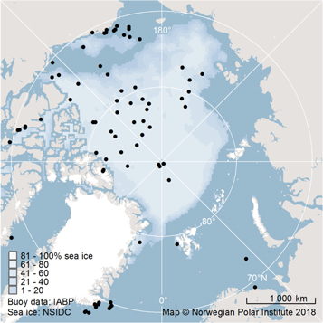
Information on snow thickness over Arctic sea ice is crucial, since snow strongly affects thermodynamic ice growth, melt pond formation, and radiative transfer. Information on snow thickness on Arctic sea ice is still sparse, although the amount of data has increased recently due to new in situ, airborne and satellite surveys (e.g. Laxon et al 2013, Renner et al 2014, Haas et al 2017, Rösel et al 2018). Reanalysis data can fill in where observations are lacking, but intercomparisons with in situ measurements have shown that they do not always match well (Boisvert et al 2018). Autonomous buoys with snow thickness sensors (ultrasonic sensors or active thermistor chains as used in IMBs) give quantitative time series data with a higher temporal resolution, and usually with a smaller footprint than airborne and satellite surveys (e.g. Brucker and Markus 2013, Maaß et al 2013, 2015). These instruments can directly measure changes in ice thickness and delineate surface and bottom melt (Perovich and Richter-Menge 2015). However, to collect representative data for a region requires many buoys. So far, the total amount of buoys at a given time in the Arctic is still rather limited, and the distribution often not very regular, so that vast areas might be without buoys at a given time (figure 2). Initiatives such as the International Arctic Buoy Programme (Rigor et al 2016, 2000) help coordinate deployments of sea ice buoys. Sophisticated buoy setups that combine measurements related to surface energy and mass balance have been developed recently (e.g. Jackson et al 2013, Wang et al 2014, 2016, Hoppmann et al 2015), as well as buoys that float and have the potential to 'survive' a regional ice-free summer (see e.g. Polashenski et al 2011). Such new developments will contribute to denser and accurate autonomously collected sea ice datasets. Understandably, relatively cheap drifter buoys with GPS but not much other sensors are the most frequent buoys used in the Arctic, while more sophisticated and multi-sensor setups are relatively rare. However, for collecting information on sea ice thermodynamics more ice mass balance buoys (IMBs) would be necessary, along with global data archives where all respective data would be accessible for the scientific community.
Figure 2. Map with International Arctic Buoy Programme (IABP) drifting buoys for mid August 2018. Vast areas of the sea ice covered Arctic have no or only sparse buoy placements. Buoy data: IABP (http://iabp.apl.washington.edu/). Sea ice concentration for 14 August 2018: National Snow and Ice Data Center (NSIDC; Brodzik and Stewart 2016).
Download figure:
Standard image High-resolution image
Recent Arctic expeditions have made increased use of new technology with mobile sensor platforms. These include autonomous underwater vehicle, unmanned airborne vehicle, remotely operated vehicle and instrument sledges. Some of these systems are still at the development stage, but with new systems becoming standard tools, it will be possible to obtain high quality sea ice data over larger spatial scales in the near future. There are still fewer in situ sea ice surveys undertaken in winter months than summer months, but recent (Granskog et al 2016, 2018, Assmy et al 2017, Rösel et al 2018) and planned interdisciplinary expeditions (e.g. the Multidisciplinary drifting Observatory for the Study of Arctic Climate (MOSAiC), www.mosaicobservatory.org) are adding to the existing winter data and providing insights into the changing Arctic sea ice system.
Ice age, also often used as a climate indicator (e.g. Perovich et al 2018, Stroeve and Notz 2018) is now less correlated with ice thickness than it used to be (Tschudi et al 2016a), since the older ice classes have become thinner. First-year ice with little snow cover can reach a thickness similar to second-year ice (Notz 2009), which has also been found in a recent field experiment in the Arctic Ocean (Granskog et al 2016). This can be a challenge for deriving ice classes from ice thickness data (Hansen et al 2014). Distinguishing first- and second-year ice by means of its thickness was probably also not always trivial previously, and is complicated using satellite microwave radiometry as well (Comiso 2006), but in total the range of thicknesses has become narrower, with the thickest ice classes becoming rare, making this more difficult. Assessing the age of ice can be supported by information on its physical properties, for example via their signature in satellite microwave scatterometry (Belmonte Rivas et al 2018), or by tracking ice movement over time (Tschudi et al 2016a). The Lagrangian tracking of ice parcels used here is subject to errors in the motion tracking, especially for regions with high spatial variability in ice dynamics, types and age within the tracked ice parcels which triggered attempts for a revision of the sea-ice age retrieval method (Korosov et al 2018). But the general good agreement between the ice age fields and ice thickness and multi-year ice extent estimates (Maslanik et al 2011) make this pan-Arctic dataset still a valuable tool to assess sea ice age on large spatial scales.
The Lagrangian ice age fields are derived from sea ice motion products (e.g. Lavergne et al 2010, Tschudi et al 2016b), which use feature tracking algorithms to estimate sea ice displacement in satellite imagery. The most commonly used source is passive microwave because of its all-sky capability. However, the low spatial resolution is a significant limitation on the precision and accuracy of the estimates and important small-scale features such as lead formation and ridging cannot be detected. The growing catalogue of SAR sensors has the potential to routinely provide daily, near-Arctic wide coverage at much higher spatial resolutions (e.g. RADARSAT Constellation), though the passive microwave record will still be valuable for long-term context.
Scientists are monitoring and studying sea ice as it drifts through Fram Strait, the area between Greenland and Svalbard, a major gate and only deepwater connection connecting the Arctic Ocean to the other world oceans (Kwok et al 2004, Spreen et al 2009, Smedsrud et al 2011, Hansen et al 2013, Renner et al 2014, Smedsrud et al 2017). Through this gate, most of the sea ice that is exported from the Arctic Ocean passes through here. Findings from here can give information on a larger area 'upstream' (Kwok 2009, Hansen et al 2013, Krumpen et al 2016). With current technology and infrastructure, continuous monitoring at such gates is only possible with moored instruments (e.g. upward looking sonars for measuring sea ice draft), satellite remote sensing, and local meteorological information. Crucial gaps in this context are or can be that there are only few or no observation sites at a gate, and potential data gaps due to instrument failures. Additional limitations arise from current remote sensing capabilities for studying the complex dynamics at such gates and a mis-match in the spatial resolution of the applied data sources (e.g. Ricker et al 2018). Given the large across-strait variability in sea-ice type, thickness and motion, SAR-based estimates of the sea-ice motion are possibly the best way to proceed (Smedsrud et al 2017) provided enough in situ data, e.g. from buoys, allow continued evaluation.
2.5. Sea-ice thermodynamics, age and dynamic processes uncertainties
Information about ice thermodynamics with high temporal resolution is often retrieved from IMBs and in situ measurements. Uncertainties are related to the question how homogenous the ice cover is, or in other words how representative a IMB site is for the region it is placed in. Depending what technology in IMBs is used, detection of snow ice and superimposed ice might be not trivial, and this can lead to an overestimation of the snow thickness and an underestimation of the ice thickness.
Drifter buoys with iridium transmitted GPS positions have a better accuracy than Argos-based buoys without GPS earlier, but ice motion can be underestimated due to motion with changing drift direction between individual position recordings. For avoiding that, we recommend position recordings at least once an hour. Sophisticated methods have been developed that use iridium transmission GPS beacons to examine sea ice motion following methodology developed for atmospheric dynamics (e.g. Lukovich et al 2015). Methods of floe tracking from satellite products are well suited to local and regional scale motion tracking (e.g. Komarov and Barber 2014, Itkin et al 2018) and detection and modelling of sea ice hazards to marine navigation (e.g. Barber et al 2014). A key gap is to develop an improved understanding of sea ice dynamic growth as a function of sea ice ridging and rubbling. Essential for this is also improved information on the spatial distribution and variability of surface roughness. The process of dynamic growth is expected to result locally and regionally in thicker ice classes even though thermodynamic growth will be reduced (see case study in Itkin et al 2018).
2.6. Biological implications of changing sea ice; uncertainties and gaps in knowledge
Knowledge and data gaps continue to limit the certainty of predictions concerning how the ice-associated ecosystem and its coupling to the pelagic and benthic food webs will respond under a changing climate. The relative ease of accessing coastal landfast ice versus the central Arctic ice-pack has resulted in biogeochemical observations being focused in key locations around the periphery of the Arctic Ocean, leaving large data gaps for vast areas of the shelves and central basins (e.g. Leu et al 2015). Similarly, logistical considerations, as well as a focus on the biologically productive period, have skewed the seasonal observational base towards spring-summer when environmental conditions are more favorable to field studies. The few autumn–winter studies that do exist (e.g. Niemi et al 2011, Niemi and Michel 2015, Assmy et al 2017, Melnikov et al 2016, Olsen et al 2017) reveal interesting ecological features of the ice-associated ecosystem, calling for a better characterization of biogeochemical processes during this time of year. Little remains known about the distribution and bloom development of sub- and under-ice primary producers and there are few within-ice primary production estimates.
Baseline information on multi-year sea ice communities encompassing biomass, productivity and biodiversity, and role in the cycling of carbon and other elements, is also an important knowledge gap which requires urgent attention given the rapid decline in Arctic multiyear ice. With multiyear ice potentially being more productive than traditionally assumed (Lange et al 2017), there is a critical need for rate measurements in multiyear ice. The likelihood of changing ice and ocean conditions enhancing the potential for toxin-producing algal blooms in the Arctic highlights a need for a better understanding of the presence, distribution, and recurrence of these species and their influence on Arctic food webs, as well as a need to improve the reporting of toxin occurrences across the Arctic. Repeat observations of higher trophic levels are also required, including fishes and marine mammals, in order to constrain their ecological responses and distributional changes in relation to the changing sea-ice cover.
Owing to the interacting effects of light and nutrients as the main factors controlling primary production at the sea ice interface and under the ice, uncertainties associated with observations and projections of the physical variables by which they are controlled, confound the capacity to predict the future structure and function of the sea-ice ecosystem. On Arctic shelves, sea ice and sea ice export contribute significantly to structure spatially diverse productivity regimes, also influenced by nutrient inventories and dynamics (Michel et al 2015, Tremblay et al 2015). As these different productivity regimes respond differently to on-going and future Arctic change (Ardyna et al 2011), a key challenge remains in resolving meso- to large-scale heterogeneity across the shelves and basins, for primary production estimates. In addition, poorly constrained estimates of the contribution of ice algae and phytoplankton to primary production and transfers to the food web, including harvest resources, require further attention. Furthermore, these uncertainties increase when predicting the responses at higher trophic levels, due to the added complexity of interactions at the species, population, community and ecosystem level.
Beyond gaps connected with sea ice ecosystem observations, it is important to mention that there is also a rather limited amount of modelling studies that address both the complexity of the physical system, and the wide range of components of the ecosystem (e.g. Duarte et al 2015, 2017).
3. Changes of gaps over time
In table 1, we give an overview on Arctic sea ice observation gaps. Some gaps disappear, while new ones emerge. This is expected and connected to both the change in sea ice conditions and processes, and in the research and monitoring activities scientists develop. New methods, designed to fill gaps, require proper validation and development in order to produce accurate data with high temporal and spatial resolution. Changing sea ice conditions result in changing knowledge needs. For example, certain processes can become less important while new, not yet fully understood processes can become relevant. Additionally, ice conditions can go beyond known examples, such as when new record low ice extents are registered, and regions become ice free, or change from perennial to seasonal ice cover. Because of this, it is critical to avoid potential gaps, for example in the passive microwave satellite record, to continue research to enhance knowledge and understanding, and to extend observations to better characterize the spatial heterogeneity of conditions. Redundancy in observation systems is also desirable. Previous assessment reports treated gaps of knowledge with varying levels of depth.
Table 1. Overview on observation gaps for Arctic sea ice.
| Parameter | Method | Gap |
|---|---|---|
|
||
| Ice extent | Passive microwave satellite sensors |
|
|
||
| Ice extent (high spatial resolution) | SAR satellite sensors | No Arctic-wide coverage as for passive microwave |
| Sea ice concentration | SAR and passive microwave, optical satellite RS | Spatial resolution, data processing algorithms, changing sensors, unclear uncertainty |
|
||
| Sea ice thickness | Satellite-based altimeters |
|
|
||
|
||
| Snow thickness | Satellites, airborne, in situ | Generally too few data |
| Sea ice mass balance | Autonomous buoys | Too few buoys running at a given time, large gaps with regions without buoys |
| Sea ice temperature | Autonomous buoys | Too few buoys running at a given time, large gaps with regions without buoys |
| Ice age | Ice thickness (all methods) | Ice age can be less easy derived from ice thickness, because ice thicknesses for different ice ages can be more similar now than earlier |
| Ice drift speed | Floe tracking, buoys | Data might be biased towards underestimating speeds; few buoys in parts of the Arctic |
| Biogeochemical and ecosystem properties and projections | Methods that depend on sea ice physics data and biogeochemical observations |
|
| Sea ice pollution | In Situ/sampling and remote sensing | Large spatial gaps of observation, and methods developed parallel to new pollutants coming up |
| Various parameters | Autonomous mobile and remote sensing based platforms | New platforms give new datasets, but calibration and validation is needed |
| Various physics and ecosystem parameters | Various methods | Lack of winter in situ data |
In the ACIA report (2005), sea ice related gaps of knowledge were not addressed specifically. However, there were more general statements made that more observations, process studies and monitoring would be necessary; sea ice freezing and melting was mentioned. Recommendations included more use of autonomous platforms, improved physics-ecosystem modelling, and establishing of data bases. Parts of these recommendations were followed up, but for most of them there is still a way to go. Several international collaborations, for example those that were a part of the International Polar Year 2007–2009 led to more observations, interdisciplinary approaches, and modern technological solutions.
The fifth assessment report of the IPCC (Vaughan et al 2013) discussed gaps in the observation record of sea ice extent, and the approach to use climatology data to fill gaps in the time series for times prior to the passive microwave satellite era (prior to 1979). This gives insights into a longer time series, but it also increases the uncertainties and size of error bars of these earlier periods 1870–1953 (twice) and 1954–1978 (factor 1.5), relative to the period from 1979 onwards. The frequent use of sea ice extent data from passive microwave satellite observations as an indicator of climate change illustrates the need to improve these datasets, to better characterize the uncertainties, and to ensure continuation of the observation time series.
The first AMAP SWIPA report from 2011 (AMAP 2011) addresses several of the gaps that were also a subject of the most recent SWIPA report (AMAP 2017). This is not particularly surprising since there was only about six years between the two reports. The lack of basin-wide snow thickness measurements was highlighted already. Ice thickness data from satellite sensors was still in development; at the time of SWIPA 2011, the methods were not yet ready for routine use. As detailed above, there is still some way to go, but the situation has improved. Several newer publications deal with use of satellite-based altimetry data (e.g. Laxon et al 2013, Kurtz et al 2014, Ricker et al 2017, Tilling et al 2018, Paul et al 2018), and one has more insights into the nature of the data received. In September 2018, the NASA laser altimetry satellite ICESat-2 was launched, likely leading to better insights into sea ice thickness distributions and changes. SWIPA 2011 also mentioned shortcomings in process understanding regarding ecosystem processes, and few long-term biological sampling initiatives/programmes. Much progress has been made but establishing long-term time-series continues to be a challenge. Some examples of current efforts include the Joint Ocean-Ice Studies in the Beaufort Sea (http://dfo-mpo.gc.ca/science/collaboration/jois-eng.html), ArcticNet in the coastal Canadian Arctic (http://www.arcticnet.ulaval.ca/), the Distributed Biological Observatory in the Pacific sector of the Arctic (https://www.pmel.noaa.gov/dbo/), MOSJ Environmental Monitoring of Svalbard and Jan Mayen (http://www.mosj.no/en/), and the Nansen Legacy in the northern Barents Sea and adjacent Arctic Basin (http://www.nansenlegacy.org). Notably, some predictions from the SWIPA 2011 report were directly addressed by the scientific community, e.g. the predicted occurrence of dual algal blooms associated with longer open water seasons, studied in Ardyna et al (2011). The upcoming MOSAiC project with fieldwork in 2019–20 will address gaps about ecosystem process understanding, and the need of more community-based observations. Community-based observing programs provide a mechanism for two-way knowledge transfers. This point was also highlighted in SWIPA 2017.
Limitations in sea ice observations present challenges for our ability to integrate observations with models to enhance understanding. The presence of short and/or inconsistent records, inadequate spatial and temporal sampling, and challenges in estimating observational uncertainty are all problematic for the optimal use of observations to inform models. This difficulty spans across possible model applications. For comparisons to climate simulations of change, the influence of internal variability needs to be thoughtfully considered. Indeed, even when considering relatively long timeseries, such as that of the nearly 40 year passive microwave ice concentration, internal variability can play an important role (e.g. Ding et al 2017) and complicate the comparison of model simulations and observations. The challenge of quantifying observational uncertainty has implications for the useful assimilation of observations for model forecasting. The lack of adequate spatial and temporal sampling of variables like snow thickness, under-ice ecosystems, and processes that drive their variability makes it difficult to use these observations to improve the model representation of relevant processes. In general, given that gaps and limitations in observations will always be present, there is a need for better methods to integrate observations and models, which explicitly consider the limitations inherent in both the observations and the models.
Traditional knowledge, for example from Inuit, can provide important value-added content to data products and serves to make the data more relevant to northern users. The Inuit have for millennia used the sea ice as a travel corridor, a platform for resource harvesting and a key cultural icon for their way of life. Closer ties are beginning to form, where the western science approach is integrated with Inuit knowledge (e.g. Krupnik et al 2010), beginning at the start of the research process and working hand-in hand through to conclusion and reporting (e.g. Barber and Barber 2009).
The fact that gaps of knowledge are more explicitly discussed recently might also reflect that there is more awareness about the relevance and importance of topics and aspects that are not fully covered and solved within the current status of knowledge.
4. Future, perspectives and strategies to reduce gaps
Some options to reduce gaps are discussed in the previous section. Although knowledge gaps will always exist, a better understanding of the Arctic sea ice system will provide a better knowledge base for decision makers to choose options for sufficient protection and sustainable management.
Uncertainties arise in the development of new methods. However, once these methods are fully developed, they help to close knowledge and observation gaps, as it is the strategy with new satellites (e.g. ESA Sentinels, NASA ICESat-2). More and more available SAR satellite data (e.g. through Sentinel) with higher resolution than passive microwave and different polarisations can help to create and support almost daily improved Arctic wide ice extent datasets in the near future, to be useful for operational purposes, validation and climate research.
In some cases, rapid progress can be made to address knowledge gaps. For example, the recent awareness about microplastic pollution in sea ice has led to upcoming research. And while insights into processes, amounts and distribution are currently rather limited, first studies do indicate substantial levels and motivate future work (Obbard et al 2014, Peeken et al 2018).
Large international efforts and projects such as MOSAiC will provide more interdisciplinary datasets in current sea ice regimes especially for seasons with few existing observations (autumn, winter). Better access to the Arctic can be a result of both new and more platforms and ships and also changing ice conditions. In general, more information and data about Arctic sea ice is essential to close gaps: this concerns new data to be collected, also through more community-based observations including automatic sensors on commercial ships and aircrafts, but also better access to existing data via data portals and data bases. The value of the data also depends on consistency of datasets collected by different groups and in different regions. Efforts to coordinate future expeditions and data collection in a more sophisticated way will help to increase the possibilities of data use and intercomparability. This includes also considering possible future datasets, to be collected with methods that do not yet exist. Archiving sea ice, snow and water samples can allow for later analysis with improved or refined methods future technologies that do not exist yet.
Communication between scientists through publications, modern social media, international projects and symposia is and will be important. Building integrated, interdisciplinary communities of modelers, field observers, and remote sensing research is a critical component of future efforts. Models can be used to inform observational strategies. The observations can then be used to improve parameterizations used in models. This approach is necessary in order to develop a new generation of creative sea ice scientists, developing projects to address crucial gaps of knowledge.
Acknowledgments
We thank five anonymous reviewers for their valuable and constructive comments on an earlier version of this paper. We are grateful for the efforts of the contributing authors to sea ice chapter in the Snow, Water, Ice and Permafrost in the Arctic (SWIPA) 2017 report, and we thank the Arctic Monitoring and Assessment Programme (AMAP) and its secretariat for coordinating the work for that report, from which the sea ice chapter represents the base for this publication. We thank Anders Skoglund, Norwegian Polar Institute, for support producing the map in figure 2. The project ID Arctic, funded by the Norwegian Ministries of Foreign Affairs and Climate and Environment (programme Arktis 2030) supported the collaboration of authors from Norway, Canada and USA. Zhijun Li's contribution was supported by the Global Change Research Program of China (2015CB953901). Marika Holland's contribution was supported by the National Center for Atmospheric Research, which is a major facility sponsored by the U.S. National Science Foundation under Cooperative Agreement No. 1852977.