

Abstract
The warm Arctic-cold Eurasia (WACE) pattern of surface air temperature anomalies is a prominent feature of the Eurasian climate variations during boreal winter. The interannual WACE anomalies are accompanied by sea ice loss in the Barents-Kara (BK) seas, however, the causality between them remains controversial because of large internal atmospheric variability over subarctic Eurasia in winter. Here we disentangle the contribution of BK sea ice loss to the WACE anomalies based on a statistical decomposition approach. An anticyclonic circulation anomaly over subarctic Eurasia that forces the WACE anomalies is found to reach its peak 3 d prior to BK sea ice loss. After excluding this prior atmospheric forcing signature, the East Asian cooling matures about 15 d later as a result of the weakened moisture transport associated with the enhanced BK downstream ridge and East Asian trough due to BK sea ice loss. The results suggest that BK sea ice loss contributes ∼65% and ∼81% of the WACE-related East Asian cooling and Arctic warming at interannual timescale, respectively, whereas the WACE-related cooling over central Eurasia primarily results from internal atmospheric variability. Such submonthly lagged East Asia cooling caused by BK sea ice loss could be helpful in predicting winter extreme cold events over East Asia.
Export citation and abstract BibTeX RIS

Original content from this work may be used under the terms of the Creative Commons Attribution 4.0 license. Any further distribution of this work must maintain attribution to the author(s) and the title of the work, journal citation and DOI.
1. Introduction
Arctic sea ice area has decreased distinctly since the beginning of satellite observations in 1979 (Comiso et al 2008, Stroeve et al 2012, Swart et al 2015, Ding et al 2017, 2022, Onarheim et al 2018, Stroeve and Notz 2018, Fox-Kemper et al 2021). Meanwhile, a warming trend of surface air temperature (SAT) has appeared over the Arctic, whereas a cooling trend and more extreme cold air outbreaks have occurred over the Eurasian continent (Liu et al 2012, Nakamura et al 2015, Screen et al 2015, Wu et al 2015, 2022, McCusker et al 2017, Johnson et al 2018, Cohen et al 2020, Rudeva and Simmonds 2021). Such a warm Arctic-cold Eurasia (WACE) dipole pattern is a prominent feature of the Eurasian climate variations during boreal winter (Overland et al 2011, Cohen et al 2012, Mori et al 2014, 2019, Kug et al 2015, Kim and Son 2016, Sung et al 2018, Luo et al 2022).
In light of apparent Arctic warming and unusual Eurasian cooling in winter during 1990–2014, some studies have focused on the decadal relationship between Arctic sea ice and WACE anomalies (Cohen et al 2014, Sun et al 2016, Dai and Deng 2022). However, it is difficult to explore causality between them at decadal timescales because of limited observations and inherent model biases (McCusker et al 2016, Ogawa et al 2018, Screen et al 2018). Meanwhile, the Atlantic Multidecadal Oscillation, the Interdecadal Pacific Oscillation and some other processes of internal climate variability have been shown to modulate the WACE at multidecadal timescales (Screen and Francis 2016, Xie 2016, Deser et al 2017), adding to the uncertainty of whether the WACE could be attributed to signals from high-latitudes. Some studies have investigated the WACE pattern corresponding to a few years of extremely-low sea ice cover in the Barents-Kara (BK) seas through composite analysis and sensitivity experiments (Cattiaux et al 2010, Petoukhov and Semenov 2010, Kim et al 2014, Wu et al 2017, Zhang and Screen 2021). Nevertheless, insufficient samplings and uncoupled experiments do not fully account for potential feedbacks that may arise in a fully coupled atmosphere-ice-ocean system (Deser et al 2016, Ding et al 2019). It remains hard to draw a solid conclusion on the relative importance of sea ice loss to the WACE anomalies.
To obtain a more general relationship between anomalous sea ice and WACE, some other studies have focused on their interannual variability (Tang et al 2013, Sorokina et al 2016, Yang et al 2016, Blackport et al 2019). Based on monthly lead-lag regressions and a physics-based approach to separate atmospheric and sea-ice forcing, Blackport and Screen (Blackport and Screen 2019, 2021) proposed that the Eurasian cooling is driven by anomalous anticyclonic circulation, not by sea ice loss. The anomalous anticyclonic circulation, which occurs simultaneously with sea ice loss and the WACE pattern, is considered to be an important internal atmospheric variability over subarctic Eurasia rather than a response to sea ice change in winter (Sun et al 2016, Blackport and Screen 2021). By contrast, some other studies have found that Arctic sea ice loss affects the mid-latitude atmospheric circulation and leads to Eurasian winter cooling by promoting similar anticyclonic anomalies (Honda et al 2009, Inoue et al 2012, Francis and Vavrus 2015, Hoshi et al 2019). Thus, the robustness of the WACE response to sea ice loss remains a subject of debate (Mori et al 2019, Blackport and Screen 2020, Cohen et al 2020, Blackport et al 2022).
As the anomalous anticyclonic circulation over subarctic Eurasia is responsible for both the reduced BK sea ice and the Eurasian cooling in winter (Kim et al 2014, Mori et al 2014, 2019, Luo et al 2016, 2019, Blackport and Screen 2019, 2021, Peings 2019, Zappa et al 2021), its response to BK sea ice loss should be singled out from its internal counterpart. Here we delineate the atmospheric response to BK sea ice loss at interannual timescale based on daily lead-lag regressions (Wills et al 2016, Wills and Thompson 2018). The atmospheric forcing of anomalous BK sea ice is linearly removed, which allows us to obtain a more robust Eurasian atmospheric response to sea ice changes.
2. Data and methods
We use wintertime (November-to-March) daily data on a 1° × 1° spacing grid for the period of 1979–2020 provided by the ERA5 global reanalysis (Hersbach et al 2020). The daily data include SAT, sea level pressure (SLP), 500 hPa geopotential height (Z500), total column water vapor (IWV), integral of water vapor transport, downward infrared radiation (IR), downward surface turbulent heat flux (THF, sensible and latent heat flux), 850 hPa temperature, wind velocity and sea ice concentration (SIC). SIC provided by ERA5 is from OSI SAF (The ocean and sea ice satellite application facility) dataset (Lavergne et al 2019), which is consistent with SIC obtained from National Snow and Ice Data Center (NSIDC; cf figures S1 and S2). Unless otherwise stated, results in this study are based on daily anomalies calculated by removing seasonal cycle and linear trend from the data. Spatial mean is computed as area-average weighted by the cosine of the latitude. To better quantify the effect of BK sea ice on the WACE anomaly pattern, we analyze the spatial mean SAT anomalies in the Arctic (65°–90° N, 0°–150° E), the central Eurasia (35°–62° N, 40°–90° E) and the East Asia (35°–62° N, 90°–135° E) regions. Following Bretherton et al (1999), the effective degrees of freedom which take the serial autocorrelation at lag 1 into account have been used in a two-tailed Student's t test for the statistical significance test of regression.
To separate the response of anomalous fields to atmospheric circulation forcing and BK sea-ice forcing in the coupled system, the following procedures are performed. (a) Wintertime daily atmospheric circulation index ( ) is defined by projecting the daily SLP field onto a SLP anomaly pattern that represents the prior atmospheric forcing of BK sea ice change (see section 3.1 for details on its construction). (b) Daily anomalous atmospheric fields at a specific time lag (
 ) are regressed on
  to obtain the regression coefficients (
 ). (c) The prior atmospheric forcing signature (
 ) is linearly removed from
  , and then a 'residue' (
 ) is used to represent the part independent of the atmospheric forcing. Here τ = 0 corresponds to the 90 day period from 1 December to 28 February in each year. The regression of
  onto the normalized winter daily time series of SIC area-averaged in the BK seas (65°–85° N, 10°–90° E) is regarded as the response to BK sea-ice forcing.
To verify the causality relationship between the WACE anomaly and atmospheric circulation forcing as well as BK sea-ice forcing, we calculated the information flow, which assumes linearity (Liang 2014). It has been used in determining the causality between rainfall and moisture divergence (Xu et al
2019) and the main factors affecting Arctic sea ice loss (Docquier et al
2022). For a pair of the time series  and
and  , the rate of information flow (in nats per unit time) from the latter to the former is given as:
where  is the sample covariance between
  and
and  ,
,  is the covariance between
  and
and  , and
, and  is the difference approximation of
  using the Euler forward scheme. A positive (negative) value of
  means that
  makes
makes  more uncertain (certain); in other words,
  increases (decreases) the variability in
  .
.
To investigate the Rossby wave energy transport over Arctic and Eurasia, we calculated the wave activity flux (WAF) according to Takaya and Nakamura (1997, Takaya and Nakamura 2001). WAF is computed as follows:
where  is the basic flow, with
  and
and  representing zonal and meridional wind velocity, respectively;
  is the background stability parameter with
  the background potential temperature and
  the specific volume;
  is the Coriolis parameter and
  is the quasi-geostrophic stream function. The primes denote the deviations from the basic flow.
To explore the role of temperature advection in the WACE-related Eurasian cooling, we calculated the temperature advection terms:

where  and
and  represent the horizontal wind vector and potential temperature at 850 hPa, respectively,
  is the climatological mean and
  is the deviation therefrom. The first term on the right hand denotes advection by the anomalous flow across the climatological-mean temperature gradients; the second term denotes advection by the climatological-mean flow across the anomalous temperature gradients; the third term denotes advection by the anomalous flow across the anomalous temperature gradients.
3. Results
3.1. Observed lead-lag relationship between BK sea ice and atmospheric circulation
In winter, SIC in the BK seas exhibits the largest interannual variability in the Arctic region (figure S1(a)). The December–January–February (DJF) mean SAT variability over Eurasia can be divided into two leading patterns by performing standard empirical orthogonal function (EOF). The first leading EOF pattern (EOF1 accounting for 35% of the total variance) shows the anomalous SAT associated with the Arctic Oscillation/North Atlantic Oscillation (AO/NAO), which has little connection with the interannual variability of BK sea ice (not shown). The second leading EOF pattern (EOF2 accounting for 17% of the total variance) shows the typical WACE anomaly pattern, with pronounced warming confined to the BK region and distinct cooling being spreading over the central and eastern parts of the Eurasian continent (colors in figure S1(b)). Therefore, the second principal component (PC2) is regarded as the WACE index. The WACE index is highly correlated with the DJF-mean SIC area-averaged in the BK seas (hereafter the DJF-mean BKsic index, dark blue line in figure S1(c)), with temporal correlation coefficient r= 0.75. However, such a high correlation does not necessarily imply that BK sea ice loss leads to the WACE pattern. Previous studies have suggested that the Eurasian anticyclonic circulation anomaly (contours in figure S1(b)), which occurs simultaneously with the WACE, is the key physical process connecting BK sea ice loss to the WACE (Luo et al 2016, 2019, Sun et al 2016, Blackport and Screen 2019, 2021, Peings 2019).
To investigate the linkages between BK sea ice and the WACE anomaly pattern, it is necessary to explore the effect of the anticyclonic anomaly on submonthly evolution. We hence defined the DJF daily time series of SIC area-averaged in the BK seas (hereafter the daily BKsic index, light blue line in figure S1(c)). The daily BKsic indices derived from ERA5 and NSIDC datasets are almost identical (r = 0.98, figure S2(a)), and have significant submonthly signals especially around 10, 15 and 30 d (figure S2(b)). We then examined the daily lead-lag regressions of SLP and SAT anomalies onto the daily BKsic index (figure 1). The daily BKsic index is always centered on the 90 day period from 1 December to 28 February, whereas the anomalous fields are regressed shifting from lag −30 d (1 November-to-29 January) to lag 30 d (31 December-to-30 March).

Figure 1. (a)–(g) Daily lead-lag regressions of SAT (colors, °C) and SLP (contours, 0.5 hPa interval) onto the normalized daily BKsic index in winter during 1979–2019, with negative (positive) lags denoting SAT/SLP anomalies leading (lagging) BKsic. Hatching indicates significance at the 90% confidence level. (h) Daily lead-lag area-mean of subarctic Eurasian (yellow box, 50°–70° N, 30°–90° E) SLP regressions (solid black line),  -related subarctic Eurasian SLP regressions (dashed black line), and Eurasian (magenta box, 35°–62° N, 40°–135° E) SAT regressions (blue line) onto the normalized daily BKsic index. The seven red dots represent the corresponding lag of days in (a)–(g). The green line in magenta box separates the central Eurasia and the East Asia.
Download figure:
Standard image High-resolution imageAs seen in the evolution of SAT anomalies from lag −9 to lag 21 (colors in figures 1(a)–(g)), the largest WACE anomalies appear around lag −3 and lag 0. The evolution of Eurasian SAT regressions shows that the most marked cooling appears at lag −1 (blue line in figure 1(h)). Meanwhile, the accompanied anticyclonic anomaly around the Ural Mountains (60° E) peaks at lag −3 (contours in figure 1(b)), which can be seen more clearly in the daily evolution of the subarctic Eurasian SLP regressions (solid black line in figure 1(h)). The evolution of Z500 anomalies (figure S3) shows patterns similar to SLP, suggesting the equivalent barotropic nature in troposphere. Such anomalous anticyclonic circulation can enhance the Siberian high and East Asian trough in winter, facilitating the transport of warm-wet air from the Atlantic Ocean to the Arctic and cold-dry air from the Arctic to the Siberia, respectively (Mori et al 2014, Overland et al 2015). This further contributes to the melting of BK sea ice and the formation of the WACE anomaly pattern. Hence, the prior anticyclonic circulation anomaly might account for most of the lagged SAT regressions onto BK sea ice.
We note that the positive SLP anomaly pattern at lag −3 is very similar to Ural blocking (e.g. Luo et al
2016, 2017, Yao et al
2017, Peings 2019, Ma et al
2022), which has been treated as an important internal atmospheric variability in winter. To represent such a prior atmospheric circulation forcing, we projected daily anomalous SLP fields onto the positive SLP anomaly pattern at lag −3 (figure S4(a), the projected subarctic Eurasian area spanning 30°–90° N, 0°–140° E) to obtain the atmospheric forcing index  (figure S4(b)). The power spectrum of
  shows significant submonthly variations with distinct spectral peaks around 14 and 30 d (figure S4(c)). As shown in figure 1(h) (dashed line), the positive SLP anomaly over subarctic Eurasian associated with
  decreases smoothly from lag −3 to lag 15, with a more negative slope from lag −3 to lag 3 compared to the decrease from lag 3 to lag 15. The evolution of
  -related SLP regression is consistent with Luo et al (2016), which found a relatively smooth decline of Ural blocking intensity during lag times using composite analysis.
However, the weakening tendency of the total anticyclonic anomaly from lag −3 to lag 21 (solid black line in figure 1(h)) is not smooth comparing to the part related to  . After a rapid decline from lag −3 to lag 3, the positive SLP regressions decrease very slowly from lag 3 to lag 15. Such abnormal evolution also exists in the Eurasian SAT (blue line in figure 1(h)). Specifically, the cooling over central Eurasia weakens from lag 0 to lag 21, while the cooling over East Asia appears to strengthen from lag 9 to lag 15 (colors in figures 1(d)–(g)). It indicates that the flattened change in anticyclonic circulation anomaly and the strengthening of the East Asian cooling are independent of the prior atmospheric forcing. We speculate that the different evolution between sea ice-related and
  -related SLP anomalies reflects the influence of BK sea ice loss, which could be masked out by the preexisting atmospheric anomalies. Next, we will investigate the contributions to the WACE anomaly from BK sea ice loss and the atmospheric internal forcing.
3.2. The atmospheric response to BK sea ice loss
To single out the atmospheric response to BK sea ice change, we use the linear decomposition described in section 2. The contributions of atmospheric forcing and sea-ice forcing are defined by regressing  and
and  onto the daily BKsic index, respectively. Figure 1(h) shows that the two peaks of Eurasian SAT anomaly occur at around lag 0 and lag 15. Here we present the SAT/SLP decomposition at lag τ = 0 and lag τ = 15 (figure 2) to better visualize the spatial structures of the different contributions of atmospheric forcing and sea-ice forcing.

Figure 2. Linear decomposition of daily lagged regressions of SAT (colors, °C) and SLP (contours, 0.3 hPa interval) onto the normalized daily BKsic index. Regressions at lag 0 and lag 15 d are decomposed into two parts: (a), (b) the atmospheric forcing part ( ) and (c), (d) the sea-ice forcing part (
 ). Hatching indicates significance at the 90% confidence level. The red boxed region (65°–90° N, 0°–150° E), the green boxed region (35°–62° N, 40°–90° E) and the magenta boxed region (35°–62° N, 90°–135° E) are used to represent the Arctic, central Eurasian and East Asian regions, respectively. (e) The area-mean SAT regressions in the Arctic region (red box) derived from lag 0 to lag 30, with lines representing for the total (black), the atmospheric forcing part (blue) and the sea-ice forcing part (red). (f) and (g) as in (e), but for the central Eurasian region (green box) and East Asian region (magenta box).
Download figure:
Standard image High-resolution imageFor the atmospheric forcing: at lag 0, the positive SLP anomaly forced by atmospheric forcing is located near the Ural Mountains (contours in figure 2(a)), accompanied by warming over the BK seas and widespread cooling over the Eurasia (colors in figure 2(a)); about 15 d later, this Arctic warming and Eurasian cooling becomes insignificant and very weak (figure 2(b)). For the sea-ice forcing: at lag 0, there is relatively enhanced warming over the Arctic region despite weaker SLP anomaly compared to the atmospheric forcing. The most remarkable difference is that the Eurasian cooling almost disappears (figure 2(c) vs 2(a)). About 15 d later, the positive SLP anomaly is enhanced and shifts to around 100° E downstream of the BK seas, with significant cooling emerging over East Asia locally (figure 2(d)).
To further look into the daily evolution of atmospheric response, we calculated the spatial-mean SAT over the Arctic, central Eurasian and East Asian regions. The Arctic warming due to atmospheric forcing is weak and disappears rapidly at positive lags, while such warming due to sea-ice forcing is remarkably larger and more persistent (figure 2(e)). It suggests that the Arctic warming primarily results from BK sea ice loss. However, the phenomenon is quite different for the cooling over the Eurasia. The contribution of atmospheric forcing dominates the cooling over central Eurasia and East Asia at lag 0, and then decreases monotonously (blue lines in figures 2(f) and (g)). In contrast to the central Eurasian cooling dominated by atmospheric forcing at all positive lags (figure 2(f)), the cooling due to sea-ice forcing plays the leading role in the East Asian since lag 10 (figure 2(g)). Specifically, the East Asian cooling due to sea-ice forcing gradually increases from lag 5 to lag 17, reaching the maximum of −0.33 °C per unit standard deviation of SIC, and then decreases (figure 2(g)). Correspondingly, the anticyclonic anomaly due to sea-ice forcing is also gradually enhanced over the BK downstream region from lag 3 to lag 15 and then weakens (figure S5). Overall, the linear decomposition suggests that the central Eurasian cooling and the anticyclonic anomaly over the Ural region that are synchronized with BK sea ice loss at lag 0 are mostly due to the prior atmospheric forcing (i.e. internal variability), while BK sea ice loss induces the East Asian cooling and the enhanced downstream anticyclonic anomaly about 15 d later. Note that the results are not sensitive to the specific domain used to define the Arctic, central Eurasian and East Asian region.
The analysis of THF further supports the above different contributions of atmospheric forcing and sea-ice forcing. The BK seas surface is dominated by downward THF anomalies at lag −3 (figure S6(a)) but upward THF anomalies at lag 15 (figure S6(b)). As seen in the evolution of THF anomalies associated with BK sea ice change, downward THF anomalies occur from 1 to 20 d before sea ice loss (solid red line in figure S6(c)). This is consistent with previous studies that downward THF anomalies over the BK seas are caused by the prior atmospheric forcing and contribute to sea ice loss (Sorokina et al 2016, Zheng et al 2022). Once BK sea ice loss is leading, the THF anomalies alter from downward to upward. This sharp asymmetry with respect to lag 0 reflects distinct atmospheric forcing of and response to BK sea ice loss. After excluding the prior atmospheric forcing, downward THF anomalies indeed disappear at all negative lags (dashed line in figure S6(c)).
In the above analysis, we attribute the anomalous SAT response to atmospheric forcing and sea ice forcing. To further prove the causality among them, we computed the information flow of atmospheric forcing ( ) and sea-ice forcing (BKsic) with SAT anomaly (figure 3), respectively. At lag 0, the information flow T(
 → SAT) has a large range of positive values over Eurasia (figure 3(a)), indicating that
  tends to increase the variability in Eurasian SAT. The information flow T(BKsic → SAT) over Eurasia is much weaker than T(
 → SAT) and mostly masked out by it (figure 3(a) vs 3(b)). However, BK sea ice clearly exerts a significant causal effect on Arctic SAT, which is not present in T(
 → SAT). At lag 15 d, BK sea ice can explicitly increase SAT variability over the Arctic and East Asia, while the atmospheric influence on Eurasian SAT largely disappears, with limited effects over vicinity of East Asian (figure 3(c) vs 3(d)). This independent analysis supports our above results that BK sea ice loss persistently drives the Arctic warming and also induces the East Asian cooling about 15 d later.

Figure 3. Information flow (a) from the  index to SAT at lag 0, (b) from the daily BKsic index to SAT at lag 0, (c) from the
  index to SAT at lag 15, and (d) from the daily BKsic index to SAT at lag 15 during 1979–2019 winter (units: 10−2 nats day−1). Hatching indicates significance at the 95% confidence level. Statistical significance is computed via bootstrap resampling with replacement of all terms included in information flow calculation using 1000 realizations.
Download figure:
Standard image High-resolution imageThe high correlation between the DJF-mean BKsic and WACE indices (figure S1(c)) motivates us to quantitatively estimate the contribution of BK sea-ice forcing to the WACE-related Arctic warming and East Asian cooling at interannual timescale. We calculated the lagged regressions of the wintertime 90-day-mean SAT/SLP fields onto the DJF-mean BKsic index (figure 4). The difference of the 90-day-mean regressions between lag 0 and lag 15 (figures 4(a) and (b)) is less than that for daily regressions (figures 1(c) and (f)), because the former excludes sub-seasonal signals. After removing the atmospheric forcing in daily fields, the Eurasian cooling largely disappears at lag 0 (figure 4(c)) and the cooling over East Asia increases to a maximum of −0.42 °C at around lag 15 (figures 4(d) and (f)), indicating that the decomposition also works for the wintertime 90-day-mean regression. The Arctic warming due to BK sea ice loss reaches a maximum of 0.97 °C (figure 4(e)). Further comparison with the Arctic warming of 1.19 °C and the East Asian cooling of −0.65 °C associated with the WACE anomaly pattern (area-mean SAT in red and magenta boxes of figure S1(b)) suggests that BK sea ice loss contributes approximately 81% of the WACE-related Arctic warming and 65% of the WACE-related East Asian cooling at interannual timescale (figures 4(e) and (f)).
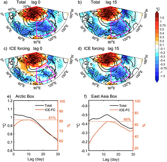
Figure 4. Lagged regressions of 90-day-mean SAT (colors, °C) and SLP (contours, 0.5 hPa interval) onto the normalized DJF-mean BKsic index. (a), (b) The original regressions at lag 0 and 15. (c), (d) As in (a), (b), but for the sea-ice forcing related regressions. Here regression at lag 15 is computed as the regression of the daily anomalous fields averaged in 16 December-to-15 March onto the 1 December-to-28 February mean BKsic index. Hatching indicates significance at the 90% confidence level. (e) The area-average SAT regressions in the Arctic red box derived from lag 0 to lag 30, with lines representing for the total (black) and the sea-ice forcing part (yellow). The horizontal line denotes the percentage of the WACE-related SAT anomaly explained by BK sea ice loss. (f) As in (e), but for the East Asia magenta box.
Download figure:
Standard image High-resolution image3.3. Mechanism for the East Asian cooling induced by BK sea ice loss
How does BK sea ice loss give rise to the East Asian cooling? To shed some light on this question, we regressed the residual parts of Z500 and 500 hPa WAF ( ) onto the daily BKsic index to represent the response to BK sea ice. As shown in figures 5(a)–(c), the propagation of wave activity from the BK seas toward East Asia is established and intensified from lag 3 to lag 15. Meanwhile, the anomalous upward stationary wave is located and enhanced over the BK seas (figures 5(d)–(f)), indicating that the stationary wave train toward East Asia is excited over the BK seas. The establishment of the anticyclonic anomaly over the BK seas and the cyclonic anomaly over East Asia in the middle troposphere could build a temperature linkage between the two regions (figure 5(c)), as suggested by previous studies (e.g. Deser et al
2004, Honda et al
2009, Inoue et al
2012, Sato et al
2014). Specifically, the anticyclonic anomaly may bring cold air from Arctic to subarctic Eurasian and thus lead to cooling therein (Honda et al
2009, Overland et al
2015). We further analyzed the 850 hPa temperature advection (
) onto the daily BKsic index to represent the response to BK sea ice. As shown in figures 5(a)–(c), the propagation of wave activity from the BK seas toward East Asia is established and intensified from lag 3 to lag 15. Meanwhile, the anomalous upward stationary wave is located and enhanced over the BK seas (figures 5(d)–(f)), indicating that the stationary wave train toward East Asia is excited over the BK seas. The establishment of the anticyclonic anomaly over the BK seas and the cyclonic anomaly over East Asia in the middle troposphere could build a temperature linkage between the two regions (figure 5(c)), as suggested by previous studies (e.g. Deser et al
2004, Honda et al
2009, Inoue et al
2012, Sato et al
2014). Specifically, the anticyclonic anomaly may bring cold air from Arctic to subarctic Eurasian and thus lead to cooling therein (Honda et al
2009, Overland et al
2015). We further analyzed the 850 hPa temperature advection ( ), and found that the significant cold air advection over Eurasia is mainly contributed by
  (i.e. advection by anomalous flow across the climatological-mean temperature gradients). But this term is only confined to the West Siberian plain (colors in figure 5(h)). Hence, the significant 850 hPa temperature cooling over East Asia caused by BK sea ice loss (figure 5(g)) is not through direct temperature advection.

Figure 5. The lagged regressions of sea-ice-related anomalous fields onto the daily BKsic index during 1979–2019. (a)–(c) Regressions of 500 hPa horizontal WAF (vectors, m−2s−2) and Z500 (colors, m) at lag 3, 9 and 15 d. (d)–(f) As in (a)–(c), but for 500 hPa vertical WAF (colors, Pa m s−2). (g)–(l) Regressions at lag 15 of the (g) 850 hPa temperature, (h) advection of the climatological temperature by anomalous flows at 850 hPa, (i) downward THF, (j) downward IR, (k) IWV, and (l) IVT. Contours and vectors in (h) represent the climatological temperature distribution and the wind regressions, respectively. Vectors in (l) represent column-integrated moisture flux. Hatching indicates significance at the 90% confidence level. The magenta box denotes the East Asia region.
Download figure:
Standard image High-resolution imageWe then turned to the downward THF and IR, which are important forcings of temperature tendency. It can be seen clearly that THF is very weak over East Asia (figure 5(i)), whereas IR exhibits significantly upward anomalies over East Asia (figure 5(j)). As IR is coupled with lower tropospheric temperature and water vapor content, the influence of IR on temperature tendency must be explored with water vapor changes. Consistent with the weakened downward IR, total column water vapor also decreases over East Asia (figure 5(k)), corresponding to the negative water vapor transport anomalies (colors in figure 5(l)). Climatologically, the wintertime water vapor over Eurasia shows eastward transport. That is, the main source of water vapor comes from the Atlantic Ocean (Luo et al 2017). Therefore, the westward moisture flux anomalies associated with the enhanced BK downstream ridge and East Asian trough due to BK sea ice loss (vectors in figure 5(l); corresponding to Z500 dipole anomalies in figure 5(c)) weaken the climatological water vapor transport, and thus the water vapor content over East Asia. Subsequently, the weakened downward IR leads to the cooling over East Asia.
3.4. East Asian cooling due to BK sea ice loss at different epochs
The decline of Artic sea ice extent in winter has accelerated since the early 2000s (Comiso et al 2008, Stroeve et al 2012, Vihma 2014, Meehl et al 2018, Ding et al 2022). Specifically, the downward trend of the DJF-mean BK SIC during 2000–2019 is about five times that during 1979–1999 (figure 6(a)). A question then arises as to whether the contribution of BK sea ice loss to the WACE-related East Asian cooling has changed accordingly or not. We further applied the decomposition analysis as in figure 2(g) but for the two epochs 1979–1999 and 2000–2019, respectively. Results suggest that the East Asian cooling affected by atmospheric forcing is significantly greater and longer during 2000–2019 than 1979–1999 (blue lines in figures 6(b) and (c)). This is consistent with the finding of Luo et al (2016) that the SAT anomalies caused by Ural blocking are more persistent after 2000. The peak of East Asian cooling caused by BK sea ice loss is almost unchanged during the two epochs, at ∼0.3 °C cooling (red lines in figures 6(b) and (c)), which is nearly identical to the value obtained for the whole period 1979–2019 (figure 2(g)). However, the shape of sea-ice forcing curve is different during the two epochs, with a progressive increase of sea-ice influence from lag 0 to lag 18 and then a decrease afterwards for 2000–2019, while there is more oscillation for 1979–1999. The difference may be attributed to climate background changes under global warming. Luo et al (2019) suggested that the climatological potential vorticity gradient over Eurasia has become weaker with a positive trend of BK air temperature due to sea ice loss, and this may lead to more persistent circulation anomalies because of weaker energy dispersion. Thus, our findings call for cautious interpretation of the results without careful filtering of atmospheric internal variability regarding the BK sea ice loss's impact on the wintertime mid-latitude weather in a warming climate.

Figure 6. (a) The DJF-mean BK SIC during 1979–2019. The slope of the linear trend of SIC is −0.13% per year for 1979–1999, and the slope is −0.67% per year for 2000–2019. The interannual standard deviation is 3.58% for 1979–1999 and 7.41% for 2000–2019. (b) and (c) as in figure 2(g), but for (b) 1979–1999 and (c) 2000–2019.
Download figure:
Standard image High-resolution image
4. Conclusion and discussion
We used a statistical decomposition approach to investigate the two-way interactions between the wintertime BK sea ice loss and the Eurasian anticyclonic circulation anomaly that forces the WACE anomalies in reanalysis data. The strongest anticyclonic circulation anomaly is found to appear 3 d prior to BK sea ice loss, suggesting that this prior atmospheric forcing may mask out the WACE anomalies in response to sea ice loss. To verify the robust atmospheric response to sea-ice forcing alone, we further analyzed daily lagged regressions of atmospheric anomaly fields after excluding the prior atmospheric forcing signature. It is found that the cooling over central Eurasian mostly disappears at lag 0 after excluding the atmospheric forcing, while the warming over Arctic is little influenced by the atmospheric forcing. The cooling caused by sea-ice forcing over East Asia would gradually increase and reach a maximum at lag 17 d. The results suggest that the winter WACE-related cooling over central Eurasia is primarily explained by internal atmospheric variability, while the warming over Arctic and the cooling over East Asia are mainly explained by sea ice loss. Quantitatively, BK sea ice loss contributes approximately 65% of the WACE-related East Asian cooling and 81% of the WACE-related Arctic warming in winter at interannual timescale. Further dynamical inspection suggests that such East Asian cooling is mainly attributed to the reduced water vapor transport associated with the enhanced BK downstream ridge and East Asian trough caused by BK sea ice loss.
The significant differences between BK sea-ice forcing regressions at lag 0 and lag 15 (figures 2(c) and (d)) are the result of strong submonthly signals in the daily fields, which allows us to distinguish atmospheric forcing and sea-ice forcing in daily lagged regressions. This cannot be achieved by applying monthly/seasonal-mean lagged regressions. It is encouraged to perform regressions at daily time-lag to look into the nature of atmosphere-ice coupling. In addition, the quantitative assessment of BK sea-ice forcing in this study is based on a linear separation of the WACE-related atmospheric forcing that is assumed to be stationary, which might underestimate magnitude and persistence of the main atmospheric internal variability and thereby its contribution to the Eurasian cooling.
We also note that sea ice change and internal atmospheric processes in autumn may have a persistent effect on following months. Previous studies suggested that sea ice loss or Ural blocking-like anomalies in autumn could lead to winter positive AO/NAO anomaly and Eurasian cooling through stratospheric-tropospheric coupling processes, but the processes are still unclear due to the high complexity (e.g. Screen et al 2014, King et al 2016, Yang et al 2016, Zhang et al 2018, Peings 2019, Chripko et al 2021, Smith et al 2022). The potential modulation of the winter Eurasian continent temperature by autumn sea ice loss and internal atmospheric variability is beyond the scope of the present study. In fact, some studies support that the winter atmospheric circulation response to sea ice loss is mainly driven by concurrent sea ice loss during winter, rather than autumn (Tang et al 2013, Blackport and Screen 2019). The ocean-to-atmosphere heat flux anomalies are most significantly affected by sea ice variability in winter (Deser et al 2010), which may act on largescale atmospheric circulation in mid-latitude through more direct physical processes.
Acknowledgments
This work is supported by National Key Research and Development Program of China (2019YFA0607001, 2019YFC1509100), and National Natural Science Foundation of China (NSFC) Projects (42276016, 41906194, 41922039).
Data availability statement
The data that support the findings of this study are openly available at the following URL/DOI: www.ecmwf.int/en/forecasts/datasets/reanalysis-datasets/era5.
Supplementary data (3.2 MB DOCX)