

Abstract
Countries are required to generate baselines of carbon emissions, or Forest Reference Emission Levels, for implementing REDD+ under the United Nations Framework Convention on Climate Change and to access results-based payments. Developing these baselines requires accurate maps of carbon stocks and historical deforestation. Global remote sensing products provide low-cost solutions for this information, but there has been little validation of these products at national scales. This study compares the ability of currently available products obtained from remote sensing data to deliver estimates of deforestation and associated carbon emissions in Guinea-Bissau, a West African country encompassing the climate and vegetation gradients that are typical of sub-Saharan Africa. We show that disagreements in estimates of deforestation are striking, and this variation leads to high uncertainty in derived emissions. For Guinea-Bissau, we suggest that higher temporal resolution of remote sensing products is required to reduce this uncertainty by overcoming current limitations in differentiating deforestation from seasonality. In contrast, existing datasets of carbon stocks show better agreement, and contribute much less to the variation in estimated emissions. We conclude that using global datasets based on Earth Observation data is a cost-effective solution to make REDD+ operational, but deforestation maps in particular should be derived carefully and their uncertainty assessed.
Export citation and abstract BibTeX RIS

Original content from this work may be used under the terms of the Creative Commons Attribution 3.0 licence. Any further distribution of this work must maintain attribution to the author(s) and the title of the work, journal citation and DOI.
1. Introduction
Land-use change accounts for 12% of global carbon emissions (Le Quéré et al 2018), and mitigation actions in this sector are strategically important under the United Nations Framework Convention on Climate Change (UNFCCC) and its Paris Agreement (UNFCCC 2016, Grassi et al 2017). Accordingly, efforts to reduce emissions from deforestation and forest degradation in tropical developing countries (REDD+) have also been high on the agenda. However, to be eligible to receive results-based payments for REDD+ efforts, countries need to fulfill certain technical requirements (Goetz et al 2015) that include establishing baselines of historical greenhouse gas emissions, or Forest Reference Emissions Levels (FREL). A FREL in UNFCCC terminology is given by the product of 'activity data' (AD) and 'emission factors' (EF), or area change and changes in carbon stock per unit of area. Existing global Earth Observation (EO) datasets for land-use change assessments (e.g. Hansen et al 2013, Sexton et al 2013, Shimada et al 2014) and of above-ground biomass (AGB) density (e.g. Saatchi et al 2011, Baccini et al 2012) may be useful in the context of REDD+ to establish emission baselines (Harris et al 2012, Achard et al 2014, Achard and House 2015, Goetz et al 2015, Tyukavina et al 2015, Zarin et al 2016). However, although EO capabilities to generate regional to global products can contribute to promote consistency and transparency across regions by tracking global progress on reducing emissions (Achard and House 2015), the suitability of these products have rarely been tested for producing baselines at national scales.
Using existing EO products is less costly than developing and maintaining operational forest monitoring systems, including the high costs of sampling, and therefore is particularly attractive to some countries with less capacity and without substantial REDD+ readiness funding (Herold and Skutsch 2011, Norman and Nakhooda 2015). However, limitations exist for their wider adoption at national and sub-national levels. Such limitations include the scarcity of studies analyzing the agreement between such products and in situ data at national and subnational scales or the differences that may be found among the available studies. For example, studies have shown that although having high overall accuracies, some products still underestimate deforestation due to confusion between forests and plantations (Tropek et al 2014, Lui and Coomes 2015) or by failing to detect small-scale disturbances (Milodowski et al 2017). These products can also overestimate tree-cover and deforestation due to discrepancies in tree-cover thresholds (Mermoz and Toan 2016, Sannier et al 2016). As for biomass, studies comparing existing pantropical maps (Hill et al 2013, Mitchard et al 2013, Mitchard et al 2014) found overall agreement and lower uncertainty when data is aggregated at larger scales, but significant differences otherwise, and thus recommended better uncertainty assessments of these pan-tropical products. Overall, these studies compared different EO products for deriving either AD or EF. However, the combined analysis of these two components, which is a prerequisite for developing national REDD+ baselines, has rarely been performed.
This study therefore assesses the impact of using different available datasets obtained with state-of-the-art automated methods based on EO data for producing a national baseline of historical carbon emissions, using Guinea-Bissau (West Africa) as a case study. With an area of ∼36 000 km2, this least-developed country is mostly covered with woodlands and mangroves (Vittek et al 2014) and encompasses the climate and vegetation gradients that are typical of many areas of sub-Saharan Africa (figure 1). We compare historical gross emissions from deforestation obtained by combining several products (for AD and EF), including nationally produced ones, and investigate (a) if consistent FRELs are derived when using different EO products; (b) if the variance is mostly due to the AD or EF component; and (c) the reasons for observed discrepancies. Overall, we wish to explore whether the concern surrounding the use of global EO products at national scales to develop REDD+ baselines is warranted.
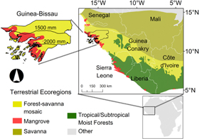
Figure 1. Map indicating the location of Guinea-Bissau in Western Africa showing terrestrial ecoregions (adapted from Olson et al 2001) and precipitation gradient (mm yr−1, WorldClim) in the Guinea-Bissau subset.
Download figure:
Standard image High-resolution image2. Data
2.1. National deforestation and AGB data
To comply with UNFCCC reporting requirements Guinea-Bissau compiled existing information on anthropogenic emissions by sources and removal by sinks in their national communications (Guinea-Bissau 2011, 2018). The main source of data for the land-use sector, including information on deforestation and forest AGB, was the CARBOVEG-GB nation-wide project which ended in 2010. This project was latter extended by the Institute for Biodiversity and Protected Areas (IBAP) with the objective of producing a baseline of emissions for the protected areas (IBAP 2015, Vasconcelos et al 2015). Information from these projects includes Landsat-based land-cover maps for 2007 and 2010 that stratify forests into four classes (table 1), and in situ AGB data collected nationwide in 309 plots (table 2). These data are referred to hereafter as the National data (see Vasconcelos et al (2015) and the appendix for detailed methods).
Table 1. The data sources used to derive deforestation estimates between 2007–2010.
| Product | References | Scale | Remote sensing data sources | Spatial resolution | Imagery acquisition dates | Description of data used to derive deforestation |
|---|---|---|---|---|---|---|
| GFC | Hansen et al (2013) | Global | Landsat | 30 m | Growing season | Tree-cover 2000 annual tree-cover loss 2000–2010 |
| GLCF | Sexton et al (2013) | Global | MODIS VCF rescaled with Landsat | 30 m | All year | Tree-cover 2005, 2010 |
| JAXA | Shimada et al (2014) | Global | ALOS PALSAR | 25 m | Growing season | Forest/non-forest 2007, 2010 |
| National | Guinea-Bissau (2011, 2018) Vasconcelos et al (2015) | National | Landsat | 25 m | Dry season | Land-cover 2007, 2010 |
Table 2. The above-ground biomass data sources used to derive emission factors.
| Product | Reference | Scale | Remote Sensing data sources | Spatial resolution | Reference year |
|---|---|---|---|---|---|
| SA11 | Saatchi et al (2011) | Pantropical | GLAS + MODIS + QuikSCAT | 1 km | 2000 |
| BA12 | Baccini et al (2012) | Pantropical | GLAS + MODIS | 500 m | 2007–2008 |
| CA12 | Carreiras et al (2012) | Guinea-Bissau | ALOS PALSAR | 50 m | 2008 |
| BO18 | Bouvet et al (2018) | African savannas | ALOS PALSAR mosaic | 25 m | 2010 |
| National | Guinea-Bissau (2011, 2018), Vasconcelos et al (2015) | 309 plots measured nationwide between 2007 and 2012 | |||
2.2. Global forest cover data
Available global datasets of tree-cover and tree-cover loss (Hansen et al 2013, Sexton et al 2013) and annual forest and non-forest cover maps (Shimada et al 2014) based on automated classification algorithms of Landsat, the vegetation continuous fields (VCF) derived from MODerate-resolution Imaging Spectroradiometer (MODIS), and Advanced Land Observing Satellite (ALOS) Phased Array L-band Synthetic Aperture Radar (PALSAR) imagery were used (table 1, and appendix). To estimate forest loss from 2007–2010, we firstly used the global forest change (GFC; Hansen et al 2013) 30 m resolution dataset based on a time-series of Landsat images from the growing season. Secondly, we used the global dataset of tree-cover made freely available by the global land cover facility (GLCF; Sexton et al (2013)). Although the final product is also a tree-cover global map, this dataset uses the 250 m MODIS VCF rescaled to 30 m resolution using Landsat data. Thirdly, we used the 25 m Forest/Non-Forest (F/NF) global mosaics for 2007 and 2010 from Shimada et al (2014) based on the Japan Aerospace Exploration Agency (JAXA) ALOS PALSAR. This product uses the lower levels of the L-band backscatter as a threshold for mapping the transition from forest to non-forest.
Table 3. Forest Reference Emission Levels (in MtCO2 yr−1) for the reference period 2007–2010 and country-wide spread given by the coefficient of variation (CV, %) for AD by fixing each AGB product, and for EF by fixing each deforestation product. The different FREL estimates are obtained as the product of Activity Data (AD, ha yr−1) derived from each dataset (National, GFC, GLCF, and JAXA) and emission factors (EF, tCO2 ha−1) obtained by each dataset (National, SA11, BA12, CA12, BO18).
| AD-GFC | AD-GLCF | AD-JAXA | AD-National | AD CV | |
|---|---|---|---|---|---|
| EF-National | 0.82 | 1.83 | 4.06 | 5.71 | 71% |
| EF-SA11 | 0.79 | 1.17 | 2.97 | 3.60 | 64% |
| EF-BA12 | 0.87 | 1.58 | 3.54 | 4.19 | 62% |
| EF-CA12 | 0.79 | 1.49 | 3.46 | 3.15 | 58% |
| EF-BO18 | 0.48 | 1.14 | 1.73 | 2.45 | 58% |
| EF CV | 21% | 20% | 28% | 32% | 64% |
2.3. AGB maps
To assess pre-deforestation carbon stocks, we used four available maps of AGB (table 2, and appendix). Two were developed at a pantropical scale (Saatchi et al 2011, Baccini et al 2012) based on transects derived from the Lidar dataset obtained by the Geoscience Laser Altimeter System (GLAS) onboard the Ice, Cloud and land Elevation Satellite (ICESat). Two additional AGB maps, based on Synthetic Aperture Radar (SAR) from ALOS PALSAR and developed for Africa savannas and dry forests (Bouvet et al 2018) and at a national scale (Carreiras et al 2012) with 25 and 50 m spatial resolution, were also used. All products used field data for calibration, and have reference years ranging from 2000–2010 (table 2). Saatchi et al (2011), Baccini et al (2012), Carreiras et al (2012), and Bouvet et al (2018) products are referred to hereafter as SA11, BA12, CA12, and BO18 respectively.
Table 4. Spearman's rank correlation coefficient between per-pixel mean and coefficient of variation (CV, %) for AD and AGB. Correlation values above 0.3 are in boldface; p > 0.05 in round brackets.
| AD mean | AD CV | AGB mean | |
|---|---|---|---|
| AD CV | 0.112 | ||
| AGB mean | −0.641 | (0.004) | |
| AGB CV | (0.047) | 0.216 | (−0.037) |
3. Methods
3.1. Deforestation (AD)
A spatial tracking approach was used to estimate gross deforestation over the 2007–2010 period. Firstly, F/NF layers were derived from all products. This included using a similar minimum mapping unit of 0.5 ha and tree-cover threshold of 10% to be consistent with the national forest definition (see appendix for details). The two National land-cover maps (2007, 2010) were reclassified into F/NF. For GFC, F/NF maps were generated for the years 2007 and 2010 using the 2000 tree-cover and annual loss maps; the 2000 tree-cover map was reclassified to F/NF with forest being defined as areas with tree-cover above 10%; loss in the period 2001–2007 was used to update the 2000 F/NF map and generate a 2007 F/NF map; the same approach was followed to obtain the 2010 F/NF map. For GLCF, F/NF maps were generated for the years 2005 and 2010 by reclassifying areas with tree-cover above 10% as forests in the tree-cover maps for the corresponding years. For JAXA, F/NF maps were already available for 2007 and 2010. For both National and JAXA the threshold for forest is 10% tree-cover, which is consistent with the national forest definition (FAO 2015). Finally, deforestation maps were generated by reclassifying each of the combined maps from forest and non-forest to deforestation and no-change. A common projection, extent and water mask was applied as detailed in the appendix.
3.2. Carbon assessment and EFs
Due to lack of accurate information on the fate of post-deforestation land-uses and corresponding carbon stocks, and to ensure the integrity of their FRELs, most countries (all FREL submissions except five up to December 2017) and other pantropical studies (e.g. Harris et al 2012, Achard et al 2014, Tyukavina et al 2015) chose to report gross instead of net emissions. This option is consistent with the stepwise approach for the development of REDD+ FRELs, which envisions the incorporation of better data and improved methodologies over time. In this study, we followed the same approach and estimated gross emissions, which means post-deforestation carbon stocks are assumed to be zero and any post-deforestation carbon sequestration is not accounted for. Additionally, tree AGB is the only carbon pool included. Field sampling methods were already described elsewhere (see appendix). To estimate plot-level AGB from National field data, three different equations were selected: for forest trees (Chave et al 2014), mangroves (best predictive model for mangroves from Chave et al 2005) and palm trees (IPCC 2003) (table A1). AGB obtained at plot level was extrapolated to the area of 1 ha using a dimensional scaling factor (see appendix). The National EF is the weighted average of the AGB density from all forest classes. For EFs derived from SA11, BA12, CA12 and BO18, instead of country averages, the pre-deforestation AGB was used by extracting the values from pixels identified as deforested by each deforestation product. AGB was converted to tCO2 ha−1 by using the standard carbon factor of 0.47 (IPCC 2006) and the 44/12 molecular weight ratio of carbon to carbon dioxide.
Table A1. Allometric equations used to estimate above-ground biomass of terrestrial forest species, mangroves species, and palm trees; diameter at breast height (1.3 m; DBH), height (H), wood density (ρ).
| Equation | Strata | Source |
|---|---|---|
| 0.0673 × (ρ × DBH2 × H)0.976 | Terrestrial Forest | Chave et al (2014) |
| 0.168 × ρ × DBH2.47 | Mangrove | Chave et al (2005) |
| 6.666 + 12.826 × H0.5 × ln H | Palm | IPCC (2003) (table 4.A.2, GPG-LULUCF) |
3.3. Estimating historic gross emissions from deforestation
For each combination of datasets, the product of deforested area (AD, ha yr−1) and the associated AGB (EF, tCO2 ha−1) was summed to render total annual emissions (FREL, tCO2 yr−1). Four AD (National, GFC, GLCF, and JAXA) and five EF (National, SA11, BA12, CA12, and BO18) products were used in this analysis rendering 20 FREL combinations. The spread between emissions obtained by these products was estimated using the coefficient of variation (CV, %) computed as the ratio of the standard deviation to the mean of all products. To assess the source of variation in derived FRELs, the CV was calculated across deforestation products whilst fixing each AGB product, and vice-versa, fixing each deforestation product and calculating the CV across the AGB products.
3.4. Identifying spatial patterns of agreement
Datasets were overlaid and combined to identify agreement between both deforestation and AGB products. To facilitate the visual interpretation of different spatial patterns, datasets were aggregated to a 10 km spatial resolution with each pixel representing the proportion of deforestation by area of national land (%) for AD and the mean AGB (t ha−1). Per-pixel statistics were computed including mean of all products, standard deviation and variation as a proportion of the mean given by the CV (%). The correlation between these statistical variables was assessed using the Spearman's rank correlation coefficient.
To understand the patterns of agreement between datasets we stratified the land area into four regions based on the National land-cover map (depicting Mangroves and Terrestrial Forests) stratified by climatic data (mean annual precipitation for the years 1970–2000 below or above 1500 and 2000 mm yr−1) from WorldClim (Fick and Hijmans 2017) version 2. The 20 FREL combinations and their CV (%) were calculated per region.
Table A2. In situ mean AGB density (Mg ha−1) per forest sub-class Closed-Forests (CF), Open-Forests (OF), Savanna-Woodlands (SW), Mangroves (M), and area-weighted average for total forest. Margin of error (MoE, 95% confidence) included as measure of spread. The area-weighted average AGB density is used as National emission factor after conversion from t ha−1 to CO2 ha−1.
| Strata | Number of plots | AGB density (t ha−1) | Standard deviation | MoE (95% CI) | Error (as % of mean) |
|---|---|---|---|---|---|
| Closed-Forests | 49 | 180.5 | 122.5 | 34.7 | 19 |
| Open-Forests | 120 | 86.3 | 38.7 | 11.3 | 20 |
| Savanna-Woodlands | 70 | 53.2 | 62.7 | 12.2 | 13 |
| Mangroves | 70 | 45.6 | 51.9 | 9.1 | 23 |
| Total area-weighted | 309 | 62.8 | 54.3 | 6.1 | 10 |
4. Results
4.1. AGB and EFs
The aggregated AGB mean for the entire country varies little between products (figure 2). All AGB estimates range between 54 and 65 t ha−1 (SA11 and BA12 respectively), and are similar to estimates derived from in situ data (National, 62.8 t ha−1). They are also substantially lower than the IPCC default for sub-tropical dry forests (130 t ha−1, IPCC 2006). Mean AGB densities from deforested areas tend to be lower than the aggregated national average indicating that deforestation occurs in areas of lower AGB (this is particularly evident for AD-National and true for all deforestation products except GFC in three of four AGB datasets). All AGB products show higher values in the south of Guinea-Bissau (figure 3) where patches of sub-humid forest are documented (Malaisse 1996). Some differences are observed elsewhere such as the lower densities in the North of the country in SA11, but overall variation in the AGB spatial distribution is low nationwide with 95% of 10 km pixels having a CV below 30% (figure 3).
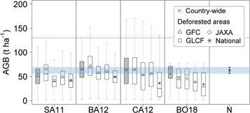
Figure 2. Distribution of above-ground biomass (AGB, t ha−1) estimates from SA11, BA12, CA12, and BO18, including minimum, first quartile, median, third quartile, maximum, and mean AGB. Estimates at the country level are highlighted in gray and the mean marked with the symbol ×. The remaining distributions describe data from SA11, BA12, CA12, and BO18 in areas mapped as deforested by each activity data product: GFC, GLCF, JAXA, and National (mean values marked with symbols Δ, □, ◊, *, respectively). Right panel depicts National (N) mean AGB (t ha−1) and the error bars the 95% confidence interval (CI) obtained from data collected nationwide in 309 sampled field plots. The 95% CI is also depicted by a blue bar for comparison with the remaining country-wide estimates. Table A3 shows mean and standard deviation values for all distributions. The National mean AGB density for the entire country (62.8 t ha−1, table A2) is used directly as proxy of pre-deforestation carbon stock or EF. The IPCC default AGB value for sub-tropical dry forests (130 t ha−1, table 4.12, IPCC 2006) is also illustrated here with a dashed line.
Download figure:
Standard image High-resolution image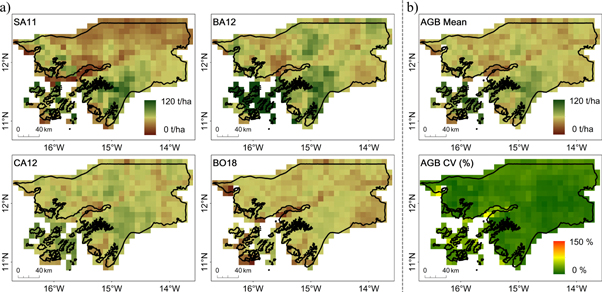
Figure 3. Spatial patterns of above-ground biomass (AGB, t ha−1) in Guinea-Bissau at 10 km resolution, including: (a) AGB distribution from different products (SA11, BA12, CA12 and BO18), and (b) per-pixel statistics including average AGB of all products and measure of spread given by the coefficient of variation (CV, %) in each pixel. The National EF is not depicted as it is estimated as the area-weighted average AGB of all forest classes with the same value of 62.8 t ha−1 used country-wide with no spatial variation.
Download figure:
Standard image High-resolution image4.2. Deforestation magnitude and spatial disagreement
In contrast to the AGB datasets, deforestation varies greatly among products with rates ranging between 0.3 and 1.8% yr−1 for GFC and National maps respectively (table A4). Even more striking are the different spatial patterns of deforestation: the different products show almost complete disagreement (figure 4). For instance, GFC identifies deforestation in the south of the country where the densest forests exist, while GLCF shows deforestation to the north in the border with Senegal and the Casamance region. Both National and JAXA highlight deforestation to the east of the country, in areas dominated by savannas, but these do not overlap. Variation as proportion of the mean (CV, %) is high to very high: over 90% of pixels have a CV above 50%.
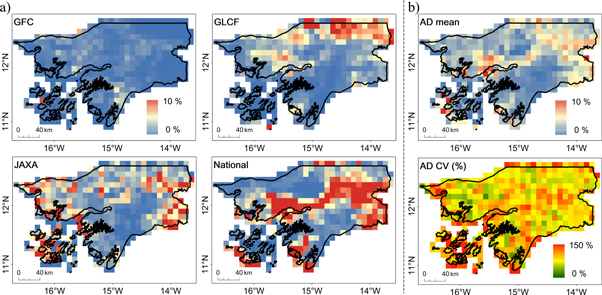
Figure 4. Spatial patterns of deforestation in Guinea-Bissau between 2007–2010 derived from different products (GFC, GLCF, JAXA and National) at 10 km resolution: (a) per-pixel deforestation values shown as the proportion (%) of deforestation by the land area of national territory (blue color denotes no change), and (b) per-pixel statistics with average and measure of spread given by the coefficient of variation (CV, %).
Download figure:
Standard image High-resolution image4.3. FREL combinations
Results for the 20 combinations of EO products show that AD and EF derived from different datasets render very different FRELs, or annual emissions (MtCO2 yr−1; table 3). Using National data produced an estimate of 5.71 MtCO2 yr−1, a value which is more than 10-times higher than the 0.48 MtCO2 yr−1 obtained when combining GFC (AD) and BO18 (EF). While the spread of all FRELs is high (overall CV of 64%), the results highlight that the magnitude of variation is dominated by differences in the deforestation dataset (AD), with CV ranging between 58%–71% when compared to the 20%–32% variation in EFs. In both AD and EF higher spread is linked to National data, while the lowest spread in AD is obtained for the two EF products derived from L-band backscatter (CA12 and BO18, 58% CV).
4.4. Relationship between spatial patterns
As suggested by the analysis of AGB densities (figure 2), there is a strong and significant relationship between higher deforestation estimates and lower AGB (table 4, Spearman's correlation 0.641; p < 0.001). There is no observed correlation between the variability of estimates of deforestation and mean AGB.
No clear relationship between different emission estimates and regions defined based on vegetation and precipitation gradient is observed either (figure 5), which was also suggested by the lack of spatial pattern in per-pixel spread (figure 4(b)). Spread in AGB is always low with slightly higher values (30%–47% CV) in forests with mean annual precipitation above 2000 mm. The spread in deforestation is always higher than that of AGB in all regions, and is particularly high in mangroves. However, mangroves are the least deforested biome and account for less than 3% of total deforestation in all datasets except JAXA, where it corresponds to 17% of total deforestation. Apart from mangrove areas, the disagreements in deforestation are not linked to specific vegetation types.

Figure 5. Country-wide and regional spread analysis given by the coefficient of variation (CV, %) in activity data (AD) and emission factors (EF). Forest types or regions (F) were stratified based on mean annual precipitation. For Mangroves the BO18 dataset is excluded, as mangrove areas are masked in the original above-ground biomass map.
Download figure:
Standard image High-resolution image5. Discussion
We produced different estimates of historical emissions from deforestation by combining pairs of deforestation and associated carbon stocks derived from different products. We show that there is a high variation in estimated emissions and that this is almost entirely due to variation in estimates of annual deforestation.
5.1. Understanding spatial disagreements in deforestation (AD)
The observed differences in the patterns and magnitude of deforestation may be linked to different imagery acquisition dates coupled with difficulties in distinguishing seasonality from deforestation. For example, the seasonality of certain crops can have a spectral signal that is difficult to separate from deforestation events without imagery from the dry season. For example, in some cases of rice plantations that have been established in previously forested mangrove areas (figure 6), images from the growing season depict a signal from swamped rice which is nearly identical to that of mangrove forest (they are 'green' from August to October). As a result, the conversion from mangrove to another land-use may be missed. However, if images are acquired in the dry season when fields are drier and the rice has been cropped (between November and July) the spectral signal will be that of bare land ('red'). In this case, deforestation events are likely to be detected. The challenge of separating the temporal spectral signal of rice production from that of conversion of mangrove forest to rice fields may have contributed to the observed higher spread in emissions in this biome (figure 5).
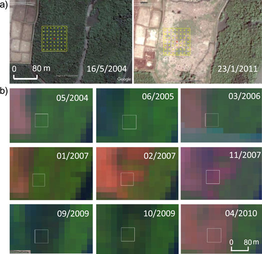
Figure 6. Example of deforestation in Mangrove through inspection of: (a) very high spatial resolution imagery available in Google Earth (16 May 2004 and 23 January 2011) showing an area of mangrove in 2004 that in 2011 was a swamped rice field; and (b) the Landsat archive with its higher temporal resolution (images ranging from May 2004 to April 2010 and displayed in RGB color composites: (b) and 7, band 4, band 3) identifying 2007 as the conversion year. The high temporal resolution of Landsat images also highlight the different spectral signals of the cycle of rice production: from August to October rice is cultivated in swamped fields (green signal) while in November the field dries out and the rice is cropped. In this study, only AD-National and AD-GLCF identified this area as deforested between 2007–2010.
Download figure:
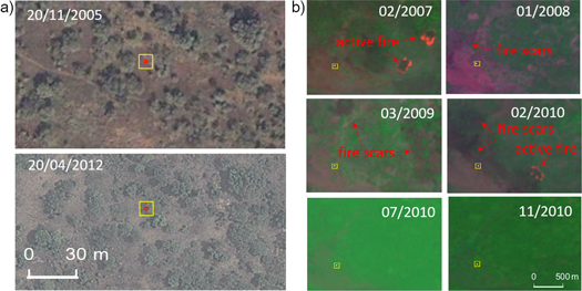
Standard image High-resolution imageThe occurrence of fire in dry biomes is another example of how seasonality may affect estimates of deforestation. African savanna fires are of low intensity and high frequency (Bowman and Murphy 2010) and in the northern hemisphere burn extensively in the early dry season (Cahoon et al 1992, Roberts et al 2009). However, typically these wildfires burn primarily grass and tree litter (Van Wilgen and Scholes 1997) and are not necessarily linked to conversion from forests to other land-uses. Consequently, the National deforestation product, relying on imagery from the dry season, may have incorrectly mapped bushfires in savannas as deforestation (figure 7).
Figure 7. Example of bushfires in Guinea-Bissau. Figure shows (a) high spatial resolution imagery from Google Earth identifying this area as forest in 2005 and remaining forest in 2012, regarding of the prevalence of fire as shown by the (b) temporal analysis of Landsat imagery with annual evidence of active fires or fire scars (displayed in RGB color composites: band 7, band 4, band 3). The area marked (yellow square) was mapped as deforested only by the AD-National product which is based on Landsat imagery from the dry season. Wildfires in African savannas typically occur in the beginning of the dry season (November–February) and their scars are very difficult to detect using remote sensing imagery from the late dry season (March–May) and growing season (June–October).
Download figure:
Standard image High-resolution image
Different acquisition dates and seasonality can therefore partially explain the lower estimates of deforestation rates in GFC and higher estimates of deforestation in National, and why, in this study, these products are associated with the lowest and highest emission estimates respectively. Importantly, there is no single acquisition date that would resolve both problems: while relying on dry season imagery is helpful for the example of mangrove conversion, this season is not suitable for detecting deforestation in fire prone areas.
While seasonality appears to be the main issue, other possibilities for the differences in estimates of deforestation can be highlighted. One is linked to the different method that was used to quantify forest loss. The GFC is the only product that detects changes by directly comparing multi-temporal images. For the remaining products, detection of deforestation was made by comparing results from independent F/NF maps, which is considered to be less accurate and may lead to an overestimation of deforestation rates (GFOI 2016). Another possible explanation for the disagreements in AD include the use of different data layers by these products. The L-band SAR backscatter has been reported to be very similar amongst mangroves, forests and plantations (Lucas et al 2014) which could explain the higher estimates of deforestation in mangroves using the JAXA product. However, the same mapping limitation is known to exist with optical data (e.g. Lui and Coomes 2015). Finally, it is also worth noting issues related with forest definitions and the complexities of using land-cover change and tree-cover change as proxy for land-use change. Although a tree-cover threshold consistent with that of national forest definition was used while processing all products, some limitations can still arise. It is considered particularly difficult to extract areas with low tree-cover densities using optical data (Achard et al 2014, Hojas-Gascon et al 2015). As a result, the use of 10% tree cover as a cut-off likely contributes to increased mapping errors and uncertainty in AD estimates. Additionally, defining forests using tree-cover thresholds fails to distinguish natural forests and plantations (Tropek et al 2014, Lui and Coomes 2015, Zarin et al 2016).
Overall, to overcome all the identified issues and map deforestation more accurately, countries would need to use very high spectral resolution imagery or increased intra-annual temporal resolution when producing their maps and estimates.
5.2. Opportunities and limitations for using available AGB datasets
While the development of EFs is considered a major monitoring capacity gap for national GHG reporting (Romijn et al 2015), our results show that for tree-AGB, using in situ data from national inventories or available datasets, even when produced at a pantropical level, render relatively similar results. Our results also highlight that the magnitude of these estimates is in all cases lower than the IPCC Tier 1 default value, with the latter leading to estimates at least 2-times higher than with other EF alternatives (table A5). Moreover, it is expected that summing AGB values over larger areas renders similar mean and total values (Mitchard et al 2013), but in our study the spatial pattern of available datasets does not differ much either. The higher spread in EFs given by the CV in forests with mean annual precipitation above 2000 mm (30%–47%) is likely not so much due to divergences in AGB products but more to limitations of data, such as the signal saturation of L-band SAR at higher levels of AGB. Nevertheless, a limitation for the use of AGB maps in baseline studies, and a possible explanation for some lower values observed in some products, is the reference year of these products. Using per-pixel AGB values as proxy for pre-deforested stock is only possible if the reference year of the AGB map precedes that of the start of the deforestation period. Finally, this study focuses only on tree-AGB, which is but one component of terrestrial carbon stocks influencing the global carbon cycle. Remote sensing products can only estimate the carbon content of other pools as a function of AGB (e.g. inclusion of below-ground biomass in Saatchi et al 2011), which is a limitation of these products for countries wanting to include emissions from other pools in their FRELs over time (i.e. in a stepwise approach). However, including other pools here as a proportion of AGB would not alter the main findings of this study.
5.3. Implications of observed differences in FREL estimates
This study finds that the variance in FRELs derived from different EO products is mostly due to the AD component. Although disagreement between products is not indicative of the accuracy of each product, it undoubtedly sheds suspicion over all products, confuses the user, and suggests producers are being overly confident in their products. While these AD products can be calibrated with reference data when developing a FREL (Olofsson et al 2014, Hojas-Gascon et al 2015), there are consequences for the use of this information in the design of appropriate policy options and REDD+ strategies. Such strategies greatly rely on understanding where deforestation is occurring and the processes that are driving land-use change. Therefore, the risk of developing the FREL independently, and possibly favouring a product with higher historical deforestation in the hope of maximizing income from REDD+ results, may be counter-productive for the success of REDD+ implementation. The two REDD+ building blocks (the FREL and REDD+ strategy) should be developed in parallel, which requires accurate spatially explicit FRELs to guide the planning of interventions. Ultimately, and considering that the availability of products for continuous global monitoring of land-use processes is only expected to expand in the future (Wulder and Coops 2014), it is important that products are carefully validated by their producers and users to quantify their uncertainty for national and subnational analysis.
6. Conclusions
Our study shows major differences are obtained in estimated emissions (FRELs) using different EO products and that those differences are mostly due to variation in estimates of deforestation. Although there are many calls for improving the accuracy of AGB maps, here we found that in situ AGB data and AGB maps relying on more sophisticated remote sensing approaches have sufficient precision for national reporting, especially when compared to the deforestation component. Divergences in the latter are striking, with almost total spatial disagreement between datasets. This finding calls for better incorporation and reporting of accuracy in land-cover (and land-cover change) EO products. In the meantime, we suggest that users focus their efforts in assessing the adequacy and quality of deforestation maps for their national circumstances by relying on reference data with higher spatial and temporal resolution to validate and calibrate existing products. Furthermore, it is also important to understand the accuracy (i.e. agreement with the truth) of those products and the causes of disagreement. This is an essential step if countries wish to use any of these products for both their FRELs and within their national REDD+ strategies to identify the drivers of change and plan activities to reduce rates of deforestation.
Acknowledgments
JBM was funded by the Natural Environment Research Council (NERC), UK, through the Leeds–York NERC Doctoral Training Partnership (grant number NE/L002574/1). G Z acknowledges the support from the European Union's Horizon 2020 Research and Innovation Programme under Grant Agreement No 641762 (Project: 'ECOPOTENTIAL: Improving Future Ecosystem Benefits through EO'). JMBC work was supported by the Natural Environment Research Council (Agreement PR140015 between NERC and the National Centre for Earth Observation). The authors thank Bouvet et al (2018) for providing their AGB map corresponding to the bounding box of Guinea-Bissau. The authors also thank the field team in Guinea-Bissau for collecting field AGB data and making these data available for this study, in particular Mr. Viriato Cassamá and Dr. Luis Catarino.
Appendix
Appendix. A.1. National deforestation and AGB data
A.1.1. Description of existing national data
Land-cover maps produced and AGB data collected under the CARBOVEG-GB nation-wide project and a subsequent project in three protected areas (IBAP 2015, Vasconcelos et al 2015) were used for this analysis and are referred throughout this study as National data. More detailed information on the production of land-cover maps, as well as field protocol and plot location is available in (Vasconcelos et al 2015).
Under these projects, Landsat TM and ETM+ images covering the entire territory of Guinea-Bissau during the late dry season in 2007 and 2010 were processed and used to discriminate four forest classes using supervised classification algorithms. The four homogeneous sub-classes of forest (Closed-Forest, Open-Forest, Savanna-Woodland and Mangrove) were aggregated into Terrestrial Forests and Mangrove to improve overall accuracy from 69%–96%.
Tree AGB data was also collected under these projects at the plot level. A 250 × 250 m stratified systematic sampling grid was created covering the entire national territory and used as a basis for plot location. In each location (randomly selected over the grid) a circular nested plot (4, 14, and 20 m concentric sub-plots) was installed following the measurement methodology described in Pearson (2005). The sampling design was stratified by forest class (Closed-Forest, Open-Forest, Savanna-Woodland and Mangrove) and a total of 492 plots were measured between 2007–2012. Several tree parameters were recorded, including diameter at breast height (DBH), height (h) and individuals identified at the species level. For some species where no wood density values were found in the literature, wood samples were also collected to estimate their specific wood density.
A.1.2. Carbon assessment of in situ data
For this study, an exhaustive process of quality control of the data led to the exclusion of plots without coordinates, plots where heights of trees were not measured, or plots with other missing information. From the entire dataset a total of 309 plots were used with 49 plots measured in Closed-Forests, 120 in Open-Forests, 70 in Savanna-Woodlands, and 70 in Mangroves. These data were compiled and analyzed here to estimate carbon densities (Mg ha−1) per forest class and total forest. For that, three different equations for estimation of AGB were selected (table A1). To estimate AGB of terrestrial forests we used the pantropical model proposed by Chave et al (2014) requiring information on tree DBH, height (H) and wood density (ρ). For mangrove species, the Chave et al (2005) common allometric equation for mangroves requiring only two parameters (DBH and ρ) was proposed due to the advantage of having used a bigger sample (n = 84) for its construction, and having more similar DBH classes than other species specific models available. No palm biomass equations were found that were specific to Guinea-Bissau, the West Africa region or even the tropics as a whole. Therefore, we selected the example allometric equation from the IPCC good practice guidance (GPG) for LULUCF (IPCC 2003) for estimating AGB of palm trees relying only on height measurements as key predictor for AGB. For both terrestrial forest and mangrove species where specific wood density was required, values from a national database were used. This database includes values from literature revision (when available) and values calculated from tree wood samples collected and analyzed under the CARBOVEG-GB project. When the species was not known or wood density values were not published/available, an average wood density was calculated from the data collected under CARBOVEG-GB (ρ ≡ 0.731 g cm−3). AGB data obtained at plot level was extrapolated to the area of 1 ha (10 000 m2) by calculating the proportion that is occupied by a given plot using a dimensional scaling factor (e), defined by the equation e = (10 000/π*r2), where r is the plot radius in meters (Pearson et al 2005). Resulting AGB estimates are shown for the sampled forest sub-classes (Closed-Forests, Open-Forests, Savanna-Woodlands and Mangroves) and for the total forest as the weighted average of the AGB density in all forest classes (table A2).
Appendix. A.2. Remote sensing datasets and methods to derive deforestation and associated emissions
A.2.1. Global forest cover datasets to derive deforestation
Available global datasets were used to derive deforestation. Firstly, the University of Maryland GFC 30 m resolution dataset based on a time-series of Landsat images from the growing season (Hansen et al 2013) was used to estimate forest cover change from 2007–2010. This product includes a global percent tree-cover map from 2000 and a map identifying the year when removal of all tree cover was observed (Hansen et al 2013, 2014). This global dataset is freely available in 10 × 10 degree tiles and the tile corresponding to Guinea-Bissau (granule with top-left corner at 20°N, 20°W) was downloaded as version 1.3 (https://earthenginepartners.appspot.com/science-2013-global-forest/download_v1.3.html). For this study only data corresponding to the period 2000–2010 was used. Therefore limitations of interannual consistency when integrating 2000–2012 data and the updated 2011–2016 data should not have any impact in our analysis. This product is thereafter referred to as GFC.
Secondly, we used the global dataset of tree-cover at 30 m resolution (Sexton et al 2013) which is freely available for download at the GLCF website (http://glcf.umd.edu/data/landsatTreecover/). This dataset uses the 250 m MODIS VCF rescaled to 30 m resolution using Landsat data. For this study we used the percent tree-cover layer for 2005 and 2010. Landsat scenes acquisition dates varied greatly (between November 2005–December 2006 for the 2005 product, and between October 2009–November 2010 for the 2010 product). As consequence, it becomes harder to compare this product to the National product that uses Landsat imagery from the dry season, or the GFC with imagery from the growing season. This product is referred to as GLCF product.
Thirdly, we used the 25 m spatial resolution Forest/Non-Forest (F/NF) global mosaics from Shimada et al (2014) based on the JAXA ALOS PALSAR. This product uses the lower levels of the L-band SAR backscatter as a threshold for mapping the transition of forest to non-forest, with forests being defined as areas of woody vegetation above 10% tree cover. Mosaics are available annually between 2007–2010 but only the maps for 2007 and 2010 were used in this analysis (http://eorc.jaxa.jp/ALOS/en/palsar_fnf/fnf_index.htm). In contrast with the GFC and GLCF products, which require a cloud screening and a stack of layers to create a per-pixel set of cloud-free observations, SAR penetrates through clouds (a unique ability when compared to optical and lidar data). Therefore it does not require cloud screening processing and multi-temporal compositing, although has been recognized these mosaics should be generated with data acquired in the dry season to avoid the impact of rainfall events (Lucas et al 2010). With this product we also do not have a reference year, but rather four independent F/NF, and two options could have been chosen for estimating deforestation. The option followed in this analysis recognizes that post-classification change detection leads to increased errors in the estimates and prioritizes having more comparable datasets. Therefore, only the F/NF maps for 2007 and 2010 were used and any deforestation captured in between is not accounted for if it regrows in 2010 (e.g. F > NF > NF > F). These mosaics covering Guinea-Bissau in 2007 and 2010 are referred to as the JAXA product. Acquisition dates are from the growing season between June–August of 2007 and from June–September of 2010.
A spatial tracking approach was used to estimate gross deforestation over the 2007–2010 temporal boundary This period was selected due to the availability of data. The processing included the following steps:
- (a)Producing mosaics from GLCF and JAXA scenes/tiles. National and GFC were already available in a single seamless raster.
- (b)Resampling all datasets to a common spatial resolution (25 m) and coordinate system (UTM Zone 28N, WGS84 datum). A nearest neighbor algorithm was used to resample all datasets to a common resolution, thus not changing the original values of each dataset.
- (c)'Water' and 'No data' were eliminated by developing and applying a common land mask. In each dataset 'water' and 'no data' were reclassified to 0 and all other values to 1. The individual land masks were then combined to produce a common binary land mask. This common land mask was finally applied to all individual datasets to exclude 'water' and 'no data' from any given product.
- (d)Generating Forest/Non-Forest (F/NF) maps. National: The two National 5-class land cover maps (Closed-Forest, Open-Forest, Savanna-Woodland, Mangrove, Non-Forest) were reclassified into F/NF maps. GFC: F/NF maps were generated for the years 2007 and 2010 using the 2000% tree-cover reclassified to F/NF with a threshold of 10% and annual loss maps in the period 2001–2007 and 2001–2010. GLCF: F/NF maps were generated for the years 2005 and 2010 by reclassifying areas with tree cover above 10% as forests in the tree cover maps for the corresponding years. JAXA: maps were already available as F/NF for 2007 and 2010. For both National and JAXA the threshold for forest is 10% tree cover, which is consistent with the national forest definition (FAO 2015).
- (e)Selection of continuous patches of forest with area equal or larger than 0.5 ha (8 pixels) to be consistent with the national forest definition of 'Land spanning more than 0.5 hectares with trees higher than 5 m and a canopy cover of more than 10 percent' (FAO 2015).
- (f)Generating deforestation maps for 2007–2010. For each product F/NF maps were combined to generate all transitions on a pixel-by-pixel basis. Deforestation maps were generated by reclassifying all possible transitions to deforestation and no-change between 2007–2010.
A.2.2. AGB datasets
We used four available maps of AGB. Two AGB pantropical maps are based on Lidar and were developed at grid scales of 1 km (Saatchi et al 2011) and 500 m (Baccini et al 2012). They used similar input data layers of sparse transects derived from the Lidar dataset obtained by GLAS onboard the ICESat before its failure in 2009. However, they are based on different field data for calibration, different data for upscaling qfrom MODIS data only (Baccini et al 2012) or MODIS and Quick Scatterometer (QuikSCAT) data (Saatchi et al 2011), and different methodologies for spatial modeling (Random Forests and Maxent respectively). Their reference year is 2000 for Saatchi et al (2011) and 2007–2008 for Baccini et al (2012). Both maps were downloaded from (the Carbon Mapper and http://whrc.org/publications-data/datasets/pantropical-national-level-carbon-stock/ respectively) and are referred to as SA11 and BA12 respectively.
The other two AGB maps used ALOS PALSAR data. Carreiras et al (2012) created a country-scale mosaic of ALOS PALSAR data from 2008 and subsequently used a machine learning algorithm (boosted regression trees) to calibrate AGB observations obtained from national field data from 2007–2008 (Guinea-Bissau 2011) as a function of ALOS PALSAR Fine Beam Dual (HH + HV polarization) backscatter intensity data to produce an AGB map for Guinea-Bissau at 50 m spatial resolution. Similarly, Bouvet et al (2018) used data from the same sensor but already in a mosaic format for the year 2010 (Shimada et al 2014) over the entire African continent. They also used in situ AGB data collected in eight African countries between 2000–2013 to produce a 25 m spatial resolution AGB map of African savannas, woodlands and dry forests. The method relies on a Bayesian inversion of a model relating ALOS PALSAR backscatter intensity as a function of AGB. Due to the saturation limitations of the L-band backscatter at higher AGB values (Collins et al 2009, Mitchard et al 2009) and its sensitivity to surface moisture conditions (Lucas et al 2010), Closed-Forests and mangroves were masked out by using the ESA Climate Change Initiative Land Cover 2010 map. Carreiras et al (2012) map and the map corresponding to the bounding box of Guinea-Bissau from Bouvet et al (2018) were made available for this study by the authors, and are referred to here as CA12 and BO18 respectively.
AGB maps were resampled to a common spatial resolution (25 m) and coordinate system (UTM Zone 28N, WGS84 datum), and a mask was applied to eliminate water values in all datasets as well as all values above 100 t ha−1 in BO18 which correspond to other classes rather than biomass (100—dense forest, 160—inundated forest, 170—mangroves, 190—urban, and 210—water; see Bouvet et al 2018 for details).
Appendix. A.3. Supplementary results
Table A3. Mean above-ground biomass (AGB, t ha−1) (± standard deviation) from SA11, BA12, CA12, BO18 (maps) and National (field plots) for the entire country and corresponding to deforested areas mapped by each activity data product: GFC, GLCF, JAXA, and National.
| Country-wide | AD-GFC | AD-GLCF | AD-JAXA | AD-National | |
|---|---|---|---|---|---|
| EF-SA11 | 55.4 (±33.0) | 65.6 (±39.1) | 42.4 (±22.7) | 50.2 (±27.0) | 42.4 (±24.1) |
| EF-BA12 | 66.4 (±25.9) | 72.0 (±29.3) | 57.6 (±19.0) | 61.1 (±24.4) | 49.7 (±18.1) |
| EF-CA12 | 62.8 (±35.9) | 63.5 (±36.5) | 53.5 (±34.5) | 55.8 (±33.3) | 36.2 (±32.2) |
| EF-BO18 | 55.4 (±21.8) | 45.4 (±21.6) | 45.5 (±22.8) | 38.6 (±21.1) | 33.5 (±24.4) |
| EF-National | 62.8 (±54.3) |
Table A4. Deforestation values and rates obtain by different products between 2007–2010.
| Deforestation rate | |||
|---|---|---|---|
| Product | Deforested area (ha) | ha yr−1 | % yr−1 |
| AD-National | 158 290 | 52 763 | 1.8 |
| AD-GFC | 22 631 | 7544 | 0.3 |
| AD-GLCF | 84 383 | 16 877 | 0.6 |
| AD-JAXA | 112 626 | 37 542 | 1.3 |
Table A5. Forest Reference Emission Level (in MtCO2 yr−1) given as the multiplication of deforestation (Activity Data, AD, ha yr−1) derived from each product (AD-GFC, AD-GLCF, AD-JAXA, and AD-National) and the above-ground biomass for tropical and sub-tropical dry forests (Tier 1, table 4.12 IPCC 2006) as pre-deforestation carbon stock or Emission Factor (EF-Tier 1).
| AD-GFC | AD-GLCF | AD-JAXA | AD-National | |
|---|---|---|---|---|
| EF-Tier 1 | 1.69 | 3.78 | 8.41 | 11.82 |