

Abstract
Urban greenhouse gas (GHG) flux estimation with atmospheric measurements and modeling, i.e. the 'top-down' approach, can potentially support GHG emission reduction policies by assessing trends in surface fluxes and detecting anomalies from bottom-up inventories. Aircraft-collected GHG observations also have the potential to help quantify point-source emissions that may not be adequately sampled by fixed surface tower-based atmospheric observing systems. Here, we estimate CH4 emissions from a known point source, the Aliso Canyon natural gas leak in Los Angeles, CA from October 2015–February 2016, using atmospheric inverse models with airborne CH4 observations from twelve flights ≈4 km downwind of the leak and surface sensitivities from a mesoscale atmospheric transport model. This leak event has been well-quantified previously using various methods by the California Air Resources Board, thereby providing high confidence in the mass-balance leak rate estimates of (Conley et al 2016), used here for comparison to inversion results. Inversions with an optimal setup are shown to provide estimates of the leak magnitude, on average, within a third of the mass balance values, with remaining errors in estimated leak rates predominantly explained by modeled wind speed errors of up to 10 m s−1, quantified by comparing airborne meteorological observations with modeled values along the flight track. An inversion setup using scaled observational wind speed errors in the model-data mismatch covariance matrix is shown to significantly reduce the influence of transport model errors on spatial patterns and estimated leak rates from the inversions. In sum, this study takes advantage of a natural tracer release experiment (i.e. the Aliso Canyon natural gas leak) to identify effective approaches for reducing the influence of transport model error on atmospheric inversions of point-source emissions, while suggesting future potential for integrating surface tower and aircraft atmospheric GHG observations in top-down urban emission monitoring systems.
Export citation and abstract BibTeX RIS

Original content from this work may be used under the terms of the Creative Commons Attribution 3.0 licence.
Any further distribution of this work must maintain attribution to the author(s) and the title of the work, journal citation and DOI.
1. Introduction
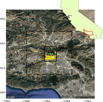
Figure 1. Leak location (green star), flux estimation domain (dashed black square), leak summation box (black rectangle, described in text) and flight tracks for all flights (yellow dots). Also shown in the inset is the leak location in California, with the red area representing the South Coast Air Basin, which has been used as a GHG estimation domain in other inverse modeling studies of southern California (e.g. Cui et al 2015). Fluxes are estimated by the inversions at a 0.005° resolution in the flux domain, resulting in a 90 × 70 matrix, or 6300 flux locations.
Download figure:
Standard image High-resolution imageCities contain a spatially-concentrated source of people and economic activity, and thus also a large source of greenhouse gas emissions. The development of effective tools to monitor greenhouse gas emissions from cities can help to enable the success of urban climate mitigation policies, e.g. those promoted through the work of the C40 network of global cities (www.c40.org). 'Top-down' methods quantify emissions by using atmospheric measurements of greenhouse gas (GHG) mole fractions to detect patterns of upwind surface fluxes. In contrast to static bottom-up inventories (based on datasets associated with fuel sales, traffic counts, electricity consumption, etc., e.g. Gurney et al 2009, Zhou and Gurney 2010), atmospheric inverse models provide the potential to supply continuous flux estimates over time, thereby detecting trends and anomalies in the bottom-up emission estimates.
Urban GHG inversion models have typically used atmospheric GHG observations (primarily carbon dioxide, CO2 and methane, CH4) from fixed surface tower networks (Kort et al 2013) to estimate spatially- and temporally-varying source fields continuously over time periods of a year or more (Feng et al 2016, McKain et al 2012, 2015, Yadav et al 2018, Lauvaux et al 2016). However, the influence of upstream fluxes on tower observations may be relatively local at times, and the towers may also miss sampling narrow plumes, or other relevant upstream sources when the wind changes direction. In contrast, aircraft measurements provide a snapshot in time of urban emissions, but with an integrated footprint higher in the atmosphere and the flexibility to adjust flight paths to directly sample known emissions locations.
Aircraft GHG data have been used previously to estimate emissions for point sources (e.g. Conley et al 2016, Lavoie et al 2015), entire cities (e.g. Brioude et al 2013, O'Shea et al 2014) or regions (e.g. Barkley et al 2017, Miller et al 2016) over short time intervals using the mass-balance (Mays et al 2009, Cambaliza et al 2014), simple scaling and inversion approaches. While mass-balance approaches, in particular, can provide estimates that are relatively accurate, most aircraft campaigns last only a couple hours, and are performed sporadically. ideally it would make sense to combine surface and aircraft data in urban GHG inversion models to help provide a more robust top-down portrait of continuous spatial and temporal emission variability.
Towards this end, we present here a small case study that aims to demonstrate the potential for using aircraft-based GHG observations in inverse models to estimate emissions from a known point source without any bottom-up prior information indicating the leak rate or location. CH4 emissions are estimated from the Aliso Canyon natural gas leak from an underground storage facility north of Los Angeles, California (figure 1), which took place from October 2015 to February 2016. An estimated 99 700 Mt of CH4 was emitted into the atmosphere during this leak event, doubling the Los Angeles basin total CH4 emissions and representing ≈20% of the state-wide budget during this time period (California Air Resources Board 2016). Multiple efforts were made to cap the leaking well, reducing emissions slowly over time from 60 Mt h−1 to 20 Mt h−1, until it was permanently sealed on 18 February 2016.
Due to the proximity of the leaking well to major population centers, and co-emitted air pollutants affecting human health during the event, the California Air Resources Board (CARB) put a substantial amount of effort into quantifying the leak rate over time using several independent methods (i.e. pressure-based calculations, aircraft mass-balance, a tracer release experiment using N2O, and ground-based remote sensing), thereby providing a high amount of confidence in their final estimates. These final estimates closely track the mass-balance values of Conley et al (2016), calculated using airborne CH4 mole fraction observations and wind speed from fourteen flights downwind of the leak from November 2015–February 2016.
The high confidence in the mass-balance estimates thereby provides a natural tracer experiment to test the quality of other modeling approaches. Here, we use the aircraft CH4 mole fraction observations from Conley et al (2016) to run atmospheric inversion models for each flight date, with measurement sensitivities to fluxes (i.e. footprints) derived from a mesoscale atmospheric transport model. By comparing inversion results to the mass-balance values, we are able to test the impact of transport model error and inversion setup choices on the resulting flux estimates. Transport model errors can be directly quantified along the flight track by comparing model output to airborne meteorological observations, which are considered to be relatively representative of upwind conditions given the small scale of the flux domain here (∼45 × 35 km).
The influence of transport model errors on atmospheric inversions are of longstanding concern, and motivated the TransCom series of global studies (e.g. Baker et al 2006, Gurney et al 2003, Law et al 2010). Transport model representations are likely to be even more problematic for observing locations in the near-field of large sources (particularly in urban areas, e.g. Boon et al 2016), than for sites in the global GHG network which were typically in remote areas sampling well-mixed air (Masarie and Tans 1995).
Approaches for reducing the influence of transport model error on urban inversions have mainly involved improving the transport model itself, or discarding atmospheric GHG observations when the associated footprints from the transport model are considered unreliable (Bréon et al 2015, Lauvaux et al 2016), e.g. for non-afternoon hours or days with complex meteorology, or even completely for sites with local influences considered difficult to model. Efforts to improve urban transport model representations have included improving the structure of meteorological models in urban areas (e.g. through the use of urban canopy models (Nehrkorn et al 2013)), or by assimilating urban meteorological observations directly to reduce biases in wind speed, wind direction and PBL height (Deng et al 2017).
However, despite best efforts to improve transport models, errors are likely to remain, as it is impossible to sample the atmosphere everywhere and all the time, and the representation of complex processes at the grid-scale are frequently imperfect approximations of sub-grid-scale phenomena. Also, discarding atmospheric observations from inversions reduces the amount of data available to constrain fluxes, and can potentially bias aggregated flux estimates by under-constraining certain portions of the underlying spatial and temporal flux variability. In complex terrain, e.g. in Los Angeles, CA, transport model errors are likely to be high, but also variable (Angevine et al 2012, Lu et al 2012). Therefore, if all GHG observations with problematic footprints were discarded from the inversion, this could potentially reduce the data constraint on fluxes to zero.
Here, we present an alternative approach for reducing the impact of transport model errors on flux estimates by directly accounting for them within the inversion itself. This approach allows us to retain all available atmospheric observations, but reduce the influence of inevitable transport model errors on flux estimates by weighting observations by the wind speed errors in their associated footprints.
Despite the impact of transport model errors and sensitivity to setup choice, inverse models can be very powerful in their ability to integrate varied data sources into a single top-down GHG observing system for urban areas. Therefore, in order to help improve the skill of urban inversions for GHG monitoring, this study has two goals: a) to reduce the impact of transport model error and optimize inversion setup for a point-scale aircraft-based inversion in complex terrain with a 'truth' for comparison, and b) to help enable the integration of aircraft and surface tower data in future work into an integrated inverse modeling system for mid- and large-sized cities like Los Angeles, CA.
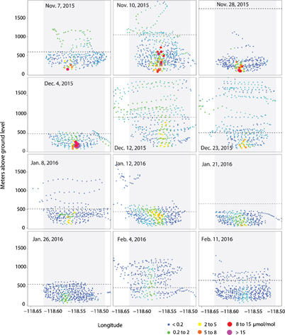
Figure 2. CH4 enhancements (observed mole fractions minus background) in vertical cross-sections (longitude vs. meters above ground level) along horizontal transects for the twelve Aliso Canyon flights analyzed here. Enhancements are shown at the 10 second average timescale. Dots are scaled by both color and size to represent enhancement magnitudes. The median planetary boundary layer height (PBL) from the WRF-STILT model (section 2.2) is marked with a horizontal dotted line.
Download figure:
Standard image High-resolution image2. Methods
2.1. Flight observational data and background air
The observational CH4 mole fraction data for the aircraft inversions is taken from Conley et al (2016), for which fourteen flights were conducted ≈4 km downwind (i.e. south) of the leaking well throughout the duration of the event in order to estimate the leak rate using the mass-balance technique. (Data collection procedures are described in more detail in appendix A.) Inversions are run for twelve flights here, corresponding to flights with published mass-balance estimates, and including only the first flight after the leak was sealed on 11 February 2016. Flight tracks for all dates are shown in figure 1, and for separate flights in figure S4 in the supplemental material available at stacks.iop.org/ERL/13/045003/mmedia.
To quantify enhancements associated with the leak, background CH4 mole fractions of air flowing into the domain (dashed black box in figure 1) must first be subtracted from the observed mole fractions. Variability in background air is assumed to be minimal relative to that of the leak enhancements, and therefore, a relatively simple approach (described in appendix A) was adopted for identifying background air mole fractions. Derived CH4 enhancements (i.e. observed—background) along vertical cross-sections of the plume are shown for each flight date in figure 2. Elevated enhancements in the center of the longitudinal transects show that the flights were able to sample directly within the leak plume for all flight dates. Maximum enhancements (at the 10 second average timescale) range from 37 μmol/mol on 4 December 2015 to just over 0.5 μmol/mol on 11 February 2016 after the leak was capped.
2.2. Transport model, footprints and transport model error
Simulated winds from the Weather Research and Forecasting (WRF) model (Skamarock and Klemp 2008, Nehrkorn et al 2010) were used here with the Stochastic Time-Inverted Lagrangian Transport (STILT) model (Lin 2003, originally based on HYSPLIT, Stein et al 2015, Stein et al 2007) to generate footprint matrices, or the sensitivity of observations to surface fluxes for the domain shown with the dashed black box in figure 1. Sensitivities were generated at a 0.005° (or ≈500 m) resolution, i.e. the flux estimation resolution for the inversions. More details on the footprint generation from WRF-STILT can be found in appendix A of the supplemental material and footprint maps for each flight date are shown in figure S4.
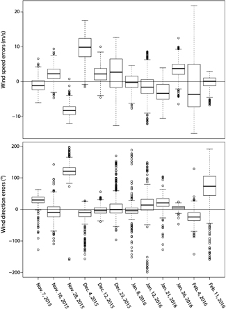
Figure 3. Boxplots of wind speed and wind direction errors (modeled WRF—observed winds at the 10-second average timescale) across observations on the flight track for each flight date.
Download figure:
Standard image High-resolution imageTransport model error was quantified along the flight track by comparing flight-based meteorological observations of wind speed and direction (Conley et al 2014) at the 10 second average timescale with WRF-STILT values. A single mean wind speed and direction error is then calculated across observations within the longitudinal extent of the plume (i.e. >0.5 μmol/mol enhancement for Aerodyne and >0.2 μmol/mol for Picarro flights, see appendix A) to compare against errors in the estimated leak rates for each flight. Errors in the modeled PBL height are also examined, as discussed further in appendix A.
Theoretically, high wind speeds (and PBLs) result in less sensitivity to the surface; hence, an over-estimated modeled wind speed (or PBL height) should result in under-estimated sensitivities and over-estimated leak rates from the inversions, that are strong enough to reproduce the observational enhancements. Similarly, under-estimated wind speeds (and PBL heights) should result in overly sensitive footprints and under-estimated fluxes.
2.3. Inversion procedure
We implement a geostatistical inverse modeling method here, where an uninformed prior flux is estimated along with a posteriori fluxes as part of the inversion (Michalak 2004, Gourdji et al 2008, Mueller et al 2008). (The geostatistical cost function minimized to estimate fluxes and their uncertainties is shown in appendix A.) This approach allows one to independently assess the atmospheric data constraint on fluxes for comparison with bottom-up inventory or process-based estimates, which are typically used as prior information in traditional Bayesian inversion approaches.
The model-data mismatch covariance matrix (or R) in an inversion describes how well the optimized fluxes should be able to reproduce the atmospheric observations, given errors associated with modeled transport, measurement and the gridded representation of fluxes. Here we assume a diagonal R matrix, i.e. uncorrelated model-data mismatch errors across observations, and test two different setups: one with a single value down the diagonal for all observations on each flight (referred to as the 'simple R'), and the second with squared observational wind speed errors (figure 3) for each observation, multiplied by a single scalar (referred to as the 'wind speed R'). The scalar value translates the wind speed errors to the same unit as the observational enhancements (i.e. μmol/mol), and provides additional flexibility to adjust the overall model-data mismatch across observations. Model-data mismatch variances are in units of ppm2, and the single variance and multiplicative scalar for the two setups are optimized using the atmospheric data, as described in appendix A.
The rationale for the second setup, i.e. the wind speed R, is that larger wind speed errors should result in larger model-data mismatch values, such that the inversion can ignore or de-weight problematic observations in its estimation procedure. This approach is similar to that of Lin and Gerbig (2005) and Lauvaux et al (2016), although simpler in implementation, given that the Lin and Gerbig method required a more in-depth analysis comparing modeled winds to radiosonde observations over the entire flux domain and additional STILT modeling to derive wind error statistics at the observation locations. Similarly, Lauvaux et al (2016) calculate transport model error statistics along the upstream footprints in a metric combining both wind speed and direction errors. Here, because our flux domain is small and includes most of the flight tracks, we assume that the observed wind speed errors for each observation along the flight track are relatively representative of the upstream footprint.
To calculate leak rates from the inversions, estimated fluxes ( ) and uncertainties () at the 0.005° estimation resolution are summed within a fixed box (figure 1, inner black box) around the actual location to derive an estimated leak rate with confidence intervals. This box is 0.06° (i.e. 12 pixels and ≈6 km) in each direction from the leak location, includes the horizontal transects flown south of the leak, and is sufficiently large to account for misplaced fluxes due to reasonable errors in both modeled wind speed and direction. In addition, the 0.12° overall width of the box corresponds to four pixels in the 0.03° flux resolution of Yadav et al (2018), which estimates fluxes for the entire Los Angeles basin during the leak, thereby facilitating future comparison between the two studies.
This box also includes Sunshine Canyon along its eastern border, a landfill with estimated CH4 emissions of ≈2 Mt h−1 (Carranza et al 2017). While these fluxes are small in comparison to emissions from the Aliso Canyon leak (from 60 Mt h−1 to 20 Mt h−1 before the leak was capped), it is likely that the mass balance estimates include emissions from Sunshine Canyon on most dates, given that the predominant observed wind direction on the flights is from the NNE (figure S3).
Finally, in order to assess how inversion setup interacts with transport model error, inversions are run for two data averaging intervals (10- and 60 second) and the two model data mismatch covariance setups (simple and wind speed R), resulting in four different setups for each flight date. The skill of the four inversions for each flight date is assessed by examining maps of flux estimates to detect correct spatial attribution of the leak emissions (section 3.2), and comparing estimated leak rates in the summation box to mass-balance reference values (section 3.3).
3. Results and discussion
3.1. Transport model errors along the flight tracks
Transport model errors are expected in the Los Angeles basin, given the difficulty in simulating atmospheric transport in the presence of the complex terrain of this area (Angevine et al 2012, Lu et al 2012), where elevations range from 200–1100 m above sea level and the ocean lies only 30 km from the leaking well in Aliso Canyon (figure 3). In this section, we analyze these errors by comparing modeled to observed wind speed and direction along the flight tracks, and then discuss the impact of these meteorological errors on the estimated leak rates from the inversions in section 3.3.
Both wind speed and wind direction errors are seen to be highly variable across the twelve flight dates, and even within a given flight, but with few systematic biases seen across flights (figure 3). Wind speeds themselves are variable, with observed median wind speeds varying from 2 m s−1 (11 February 2016) to 17 m s−1 (26 January 2016 and modeled values varying from 2–21 m s−1 (figure S3).
On 23 November and 4 December 2015, wind speed errors are particularly large, with the median modeled values 8 m s−1 too slow and 10 m s−1 too fast respectively (figure 3). This translates into error percentages of −80% and 150% for these two extreme days, and between −50% and 50% for all other flights, with roughly a third of modeled values within 25% of observed wind speeds across flights. On some dates, wind speed errors are consistently in one direction (e.g. on 28 November 2015), but on other dates (e.g. 23 December 2015 and 4 February 2016), wind speed errors are both positive and negative depending on location within the flight track. On a few dates (8 January 2016 and 11 February 2016), the median wind speed error is close to zero, and 5% of modeled values across flights have essentially no error (i.e. differences from observed values are within their reported error of 0.3 m s−1, Conley et al 2014).
Observed and modeled wind directions are predominantly from the NNE, with a median value of 15° from north (figure S3), with slightly more variability in the modeled values compared to observations. Therefore, wind direction errors (figure 3) are minimal for most flight dates, i.e. between −30° and 30° except 28 November 2015 (median of 121°) and 11 February 2016 (median of 73°), such that the modeled footprints have some sensitivity to the actual leak location for all flights except on 28 November 2015 (figure S4).
Errors in the modeled PBL height from WRF-STILT are more difficult to assess, as discussed in appendix A, although there are flight days with relatively obvious errors, as seen by comparing the plume height to the median modeled PBL (figure 2). For example, the modeled PBL height is likely too high on 28 November 2015 and too low on 4 February 2016. In fact, on this latter date, many observations in the observed plume are above the modeled PBL and therefore have little modeled sensitivity to the surface in the footprints (figure S4).
A first-order assessment of the impact of transport model error on inversion results can be obtained by transporting forward the mass-balance leak rate to the observation locations (i.e. multiplying the leak rate in the Aliso Canyon pixel by the modeled footprint sensitivity). Correlations between observed and modeled mole fractions are positive for almost all flights, but higher at the 60 second compared to the 10 second timescale, pointing to the benefits of data averaging for reducing the impacts of small-scale transport model error on flux estimates. Results from this analysis are discussed further in appendix B.
Finally, it should be noted that the transport model errors shown here near Aliso Canyon do not necessarily correspond to LA basin-wide measures of WRF model quality. A comparison of the wind speed and direction errors shown here with basin-wide metrics calculated using a network of surface observations (results not shown) showed close to zero correlation across flight dates, implying that the large errors in the Aliso vicinity, e.g. on 28 November 2015, are relatively localized problems within the domain.
3.2. Spatial patterns of estimated fluxes from inversions
Estimated fluxes are shown in figures 4 and 5 for six flight dates from the 10 second inversions with the two model-data mismatch setups in R. (Estimated fluxes from the other six flight dates are shown in supplemental figures S7 and S8.) Ten-second inversion results are shown here, since their leak emission estimates tend to be more spatially resolved than those from the 60 second data inversions, where estimated fluxes are smeared over larger areas (results not shown).
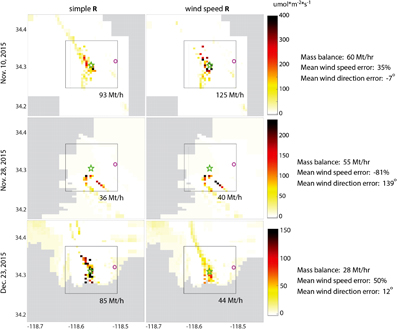
Figure 4. Flux estimates from flight inversions for 10 November 2015, 28 November 2015 and 23 December 2015 for the 10 second data resolution and a model-data mismatch covariance matrix (R) with a single variance (left) and variances proportional to squared wind speed errors (right). The box, also shown in figure 1, represents the vicinity of the leak location in which gridded emission estimates are summed to provide an estimated leak rate, indicated below the box. The actual leak location is marked by a green star, and Sunshine Canyon landfill with a magenta circle. Next to each set of maps are shown the mass-balance estimate and mean wind speed and wind direction errors inside the plume for each flight date.
Download figure:
Standard image High-resolution image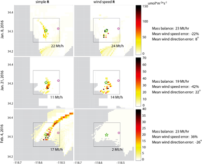
Figure 5. The same as for figure 4 for flight inversions on 8 January 2016, 21 January 2016 and 4 February 2016.
Download figure:
Standard image High-resolution imageLeak emissions are spatially allocated within the defined box for almost all flight dates for the 10 second inversions with the simple R, and on 4 December 2015 (figure S7), the inversion is able to attribute the leak to a few pixels exactly near the leak location. Even on days when the modeled wind direction errors are more than 90° (i.e. on 28 November 2015 when the footprint shows no sensitivity to the actual leak location, and 11 February 2016), most of the flux is still placed within the defined box. This is because the flight tracks themselves are within the box (figure 1), along with slow modeled wind speeds of ≈2–3 m s−1 on these days, which keeps the estimated fluxes close to the observation locations, albeit in the wrong direction from the flight track.
For three flight dates (10 November 2015, 12 December 2015, and 4 February 2016), the inversions spread part of the leak mass along the upwind plume NW or NE of the leak box. However, on two of these dates (10 November and 12 December 2015), the great majority of the leak mass is still attributed within the box. Only on 4 February 2016, the inversion smears a substantial portion of the emissions outside the box due to weak overall modeled sensitivity of observations to fluxes (figure S4).
Using the wind speed R generally helps the inversions to spatially attribute emissions to fewer pixels closer to the actual leak location (e.g. 10 November 2015, 4 December 2015 and 8 January 2016) (figures 4 and 5). The use of these wind speed errors in R changes the relative constraint on flux estimates from the observations, such that some observations have a smaller model-data mismatch (more effective weight), while others have a larger mismatch (less effective weight); this should reduce the influence of observations with larger wind speed errors (figure S6). However, it should be noted that this modified model-data mismatch can help to compensate for errors in modeled wind speed in spatially locating the leak, but not wind direction, because these two types of errors are uncorrelated in this domain.
The estimated spatial patterns can also become worse with the wind speed R, especially when observations with larger wind speed errors correspond to high enhancements within the plume, e.g. on 12 December 2015 and 21 January 2016. Also, the mean model-data mismatch (in μmol/mol) across observations can change between the two covariance matrix setups, providing an overall tighter or looser constraint on flux estimates by the observations. For example, on 23 December 2015, the mean model data mismatch goes up from ≈0.4 μmol/mol to 0.8 μmol/mol with the wind speed R, reducing the overall constraint on flux estimates and resulting in more spatially diffuse emission patterns. On 4 February 2016, the leak is no longer seen at all in the flux estimates with the wind speed R, given that the model-data mismatch becomes larger than many of the enhancements themselves, which, combined with low modeled sensitivity to the surface (because of the under-estimated modeled PBL height), resulted in no effective constraint on fluxes.
As a quantitative check on whether the spatial patterns improved from inversions using the simple to the wind speed R, we calculated the center of mass in the estimated flux maps in both the longitudinal and latitudinal directions, and then calculated the distance from the center of mass to the actual leak location for both sets of inversions. We found that the mean distance to the leak did not change by using the wind speed R, given that for a few dates, the pattern got substantially worse; however, the median distance to the leak did go down slightly from 6 to 5 km for the 10 second inversions, and from 7 to 6 km for the 60 second inversions. Also, the center of mass moved significantly closer (at 1σ) to the leak location for eight of 12 flights with the 10 second averaging, and for six flights with the 60 second averaging, while the center of mass moved significantly further away for only three and two flights respectively.
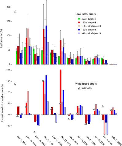
Figure 6. (a) Inversion vs. mass balance estimates (Conley et al 2016) of leak rate (Mt h−1). Mass balance and inversion estimates are both shown with 1σ confidence intervals. Inversion results are shown for four different setups: 10 second data averaging with the simple and wind speed R matrices, and 60-second data averaging with the simple and wind speed R matrices. (b) inversion error percentages (relative to the mass balance) for the four setups, and mean wind speed error percentages (comparing airborne observations to WRF-STILT values) within the leak plume.
Download figure:
Standard image High-resolution image
Figure 7. Mean errors in modeled wind speed (%) within the plume compared to estimated leak rate errors (% difference from mass balance). Results are shown for the inversions with 60 second averaging and a simple R (dark blue) vs. wind speed R (light blue). Also shown are the errors from a mass-balance calculation using WRF (rather than observed) wind speeds (green). Flight dates are labeled for outliers from the fitted line and extreme wind speed errors. The slope and r2 from a linear regression between wind speed and inversion errors for each inversion and mass balance setup are shown next to the fitted lines.
Download figure:
Standard image High-resolution image
3.3. Estimated leak rates from inversions
As expected, leak rates (i.e. summed fluxes within the box) with the simple R are over-estimated by the inversion when modeled wind speed errors are positive, and under-estimated when wind speed errors are negative for almost all flight dates (except 7 November 2015 and 4 February 2016; figures 6(a)–(b)). Moving from 10- to 60 second averaging helps to reduce estimated leak errors to some degree by averaging out high enhancements in the data due to narrow plumes which cannot be modeled properly with WRF-STILT. Using this coarser data averaging reduces the mean absolute error percentage in the leak rate across flights from 55 to 46% with the simple R.
Using the wind speed R further corrects the estimated leak rates towards the mass-balance estimates, for just half of the flights with 10 second averaging but for nine of twelve flights with 60 second averaging (with the mean absolute error further reduced from 46% to 32% with the wind speed R). For example, on 23 December 2015 with a mean wind speed error of 50%, the leak rate was corrected downwards from 85 Mt h−1 (10 second) to 59 Mt h−1 (60 second) with the simple R, and then to 38 Mt h−1 with the 60 second wind speed R (compared to 28 Mt h−1 with the mass balance). On 21 January 2016 with a mean wind speed error of −42%, the 60 second inversion was corrected upwards from 11–14 Mt h−1 with the wind speed R (compared to a mass balance estimate of 19 Mt h−1). On a few dates, the leak estimate was overly reduced with the 60 second wind speed R, i.e. for 12 December 2015 and 4 February 2016, when the data constraint on the leak was reduced by a large model-data mismatch relative to the enhancements within the plume.
The 1σ confidence intervals on the inversion leak rate estimates (figure 6(a)) are relatively wide compared to the reported uncertainties on the mass-balance estimates, and contain the mass-balance leak rate for almost all flight dates and inversion setups. This shows that the analytical uncertainties are performing well in terms of revealing the information content of the inversion flux estimates. The confidence intervals are wider with a higher leak rate for the earlier flights, and sometimes become larger from the simple to the wind speed R (e.g. on 10 November 2015, where more of the mass was placed inside the leak box with 10 second averaging), and sometimes smaller (e.g. on 4 December 2015, where the leak magnitude over-estimate was substantially corrected downwards for both 10- and 60 second averaging).
Mean wind speed errors within the plume and inversion leak rate errors have a relatively tight correlation across flights for the inversions with the simple R (figure 7), with a regression between mean wind speed and inversion errors for the 60 second averaging showing an r2 of 0.70 and a slope of 1.00 (implying a one-to-one ratio between wind speed error and inversion error percentages.) Using the wind speed R instead, the influence of wind speed errors on inversion leak rate errors is effectively reduced, with the r2 going down to 0.22 and the slope of the relationship reduced to 0.40. For the 10 second data averaging (results not shown), there is also a reduction in the influence of wind speed error on leak estimates (r2 from 0.48 to 0.21, and slope from 0.93 to 0.51), although not quite as much as with the coarser 60 second data averaging resolution. Interestingly, the wind direction errors in this study do not have any correlation with inversion leak rate errors (figure S9) for either the simple or wind speed R, given that we are summing in a relatively large box around the actual leak location that can compensate for moderately misplaced fluxes. Also, there is no prior information in the inversion that could possibly smear the flux into a larger region as a compromise between the prior and the data constraint.
Regardless, wind speed errors are not the only source of leak estimation errors here, as can be seen in figure 7 by the r2 <1 for both model-data mismatch setups. Other sources of error could be due to uncorrelated transport model errors (e.g. in PBL height), errors in the background estimation, aggregation error associated with the grid resolution, or the definition of the leak box among others. Remaining errors in the inversion leak rates, from whatever source, can potentially be further reduced by increasing the data constraint, e.g. by combining aircraft measurements with surface tower observations. (Please see appendix B for a small case study integrating nearby surface tower data with aircraft measurements for the twelve flight dates.)
Figure 7 also shows the relationship between wind speed and leak estimation errors if WRF wind speeds were used in place of actual observed wind speeds in the Aliso Canyon mass balance calculations. Observed wind speeds were used in Conley et al (2016), but modeled wind speeds are occasionally used for mass balance estimates when the domain is large and a meteorological model is needed to understand varying conditions between upstream and downstream transects (e.g. Karion et al 2015). As might be expected with mass-balance calculations that are linear with respect to horizontal wind speeds, there is an almost one-to-one relationship between modeled wind speed and mass-balance errors here, with a slope of 1.12 for the regression line. This shows that inversions, while sensitive to transport model errors that are difficult to eliminate even with a highly-tuned meteorological model, still have the potential, relative to mass balance approaches, to reduce the influence of these errors by properly accounting for them in the inversion setup.
Finally, it should be noted that using squared wind speed errors in R has the most ability to improve inversion flux estimates when meteorological errors are variable across the flight track (figure S6). If these errors are minimal, or have a consistent bias, this approach cannot de-weight some observations relative to others to reduce their overall influence on flux estimates. Systematic errors in meteorological variables are likely best corrected in the transport model itself, perhaps through surface nudging of model output to aircraft observations, or perhaps, direct modification of wind fields before input into the Lagrangian particle-tracking model (i.e. STILT in this case) for footprint generation. Correcting the influence of systematic transport model errors on inversions remains an avenue for future research.
4. Conclusions
The Aliso Canyon natural gas leak from an underground storage facility from October 2015 to February 2016 in the Los Angeles, CA basin, while an unfortunate event for the climate and public health, also provided scientists with a natural tracer experiment to help evaluate various modeling approaches for quantifying the emission rate. Here, we used the Aliso Canyon event to evaluate the ability of atmospheric inverse models, using airborne observations of the downwind plume, to spatially locate and quantify the Aliso leak on twelve flight dates throughout the duration of the leak. Inversion quality was assessed by comparing the spatial pattern of flux estimates to the actual location of the leaking well, and the estimated leak rate to the mass-balance estimates from Conley et al (2016), which were in turn validated through a multi-method comparison by the CARB. We then investigated approaches for reducing the impact of transport model error on leak rate estimates by accounting for these errors within the inversion itself.
We show here that the WRF-STILT mesoscale atmospheric transport model performed reasonably well (in comparison to airborne observations of wind speed and direction) for simulating meteorological conditions in this northern corner of the Los Angeles basin with complex terrain and land-sea breezes. Nine of 12 flight dates had mean wind speed errors within 50% of observed values, and ten of 12 flights showed mean wind direction errors within 30°.
Twelve aircraft inversions, using the simulated footprints and observed CH4 enhancements within the downstream plume, also performed remarkably well in spatially attributing the estimated emissions to a 6 km radius box around the leak site and in quantifying the leak rate within realistic confidence intervals. Wind direction errors were found to be unimportant for quantifying the leak rate within a sufficiently large box, especially with no prior information as to the actual leak location included in the inversion, and the flight tracks only ≈4 km away from the leaking well. However, errors in estimated leak rates within the summation box were found to be significantly explained by wind speed errors in the emissions plume along the flight track.
An inversion setup using scaled squared wind speed errors (i.e. modeled—observed for each observation) in the model-data mismatch covariance matrix, rather than a single variance across all observations, was found to have a large potential to reduce the impact of transport model errors on inversion results by de-weighting problematic GHG observations and their associated footprints. While airborne meteorological observations could also potentially be assimilated directly into transport models, even highly tuned transport models are computationally intensive and still subject to biases at specific points in time and space, such that an approach to directly account for transport model errors in an inversion is potentially simpler and can only help to improve the quality of flux estimates. Furthermore, the approach presented here can potentially help to retain all available atmospheric observations in an inversion, so as not to bias flux estimates by systematically discarding a portion of them, as done in other studies.
For surface tower inversions, near-surface meteorological observations at the tower locations may not as neatly represent transport model errors in the entire upstream footprint as is the case for this small-scale aircraft study. However, by comparing available observations, from both surface and airborne platforms, to modeled meteorological variables throughout the footprint, mean wind speed errors can potentially be quantified through the use of spatial interpolation approaches (e.g. kriging) before incorporation into inversion models.
Given the relatively good performance of WRF-STILT combined with an appropriate inverse model setup for estimating a point source as shown here, fine-scale models that directly resolve turbulence (e.g. the Large-Eddy Simulation model, Nottrott 2014, Prasad et al 2017) may not be necessary for simulating fine-scale variability in atmospheric dynamics around point sources. The additional benefit may not be worth the extra computational cost, depending on the desired accuracy and goals of the study, although additional research is warranted, particularly for measurements made even closer to point sources.
The approach shown here suggests the potential for integrating aircraft measurements of point source emission plumes with continuous surface tower observations in urban inverse modeling systems to help quantify and detect trends in whole-city emissions, and even evaluate spatial and sectoral patterns specified in bottom-up inventories. More informed uses of meteorological observations in inversions can also help to augment the value of GHG mole fraction measurements (collected from both surface towers and aircraft campaigns) by reducing the influence of transport model errors on final flux estimates in top-down urban inverse modeling systems.
Acknowledgments
The inversion modeling work here was supported by the NIST Greenhouse Gas Measurements Program, and the data collection was funded as described in Conley et al (2016): 'Methane emissions from the 2015 Aliso Canyon blowout in Los Angeles, CA'.