

Abstract
The Los Angeles (LA) basin was responsible for approximately 20% of California's methane emissions in 2016. Hence, curtailment of these emissions is required to meet California's greenhouse gas emissions reduction targets. However, effective mitigation remains challenging in the presence of diverse methane sources like oil and gas production fields, refineries, landfills, wastewater treatment facilities, and natural gas infrastructure. In this study, we study the temporal variability in the surface concentrations from February 2015 to April 2022 to detect a declining trend in methane emissions. We quantify the reduction due to this declining trend through inverse modeling and show that methane emissions in the LA basin have declined by 15 Gg, or ∼7% over five years from January 2015 to May 2020.
Export citation and abstract BibTeX RIS
1. Introduction
Even though there have been several published methane (CH4) emission estimates for the Los Angeles (LA) basin using various methods, vast differences exist between bottom-up, and top-down CH4 budgets. Two of these estimates are based on the bottom-up temporally invariant inventory for a single year, i.e. 2012 (e.g. Jeong et al 2013, Maasakkers et al 2016), and the remaining are the efforts that use CH4 concentration measurements from in-situ sites (aka top-down), aircraft flights, or remote sensing instruments (e.g. Wunchst et al 2009, Hsu et al 2010, Wennberg et al 2012, Peischl et al 2013, Santoni et al 2014, Wecht et al 2014, Cui et al 2015, Jeong et al 2016, Wong et al 2016, Wunch et al 2016). The combined mean CH4 emissions estimate of these studies is ∼43 000 kg h−1, with a lower bound of ∼16 000 kg h−1 and an upper bound of ∼70 000 kg h−1 (figure 1). Overall, it has been estimated that CH4 emissions of ∼43 000 kg h−1 in the LA basin account for 20% of all CH4 emissions in California (Jeong et al 2016). Note that the spatial domains of all the studies mentioned in figure 1 are inconsistent. For example, the estimates provided by Hsu et al (2010) only apply to LA County and not to the entire spatial domain of this study.
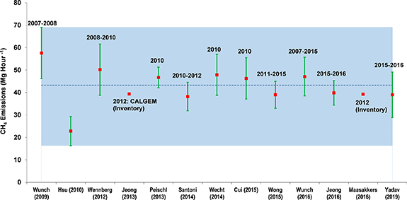
Figure 1. Annual estimates of the CH4 emissions reported in previous studies. The dashed blue line represents the mean CH4 emissions estimates across all the studies. The period for which emissions are reported is mentioned above the individual studies, and the year and the last name of the first author of the study are listed on the horizontal axis.
Download figure:
Standard image High-resolution imageTemporal trends in the estimates of CH4 emissions across multiple studies remain indiscernible, especially when we account for uncertainty in emissions. This also applies to studies performed over a longer duration (e.g. Wong et al 2016, Wunch et al 2016). Conditionally, this requires a thorough assessment of the temporal change and uncertainty through longitudinal observations obtained over multiple years from either remote sensing or in-situ platforms. Out of these two platforms, only the latter provides high-fidelity measurements with increased frequency to detect relatively small temporal changes in the variability of CH4 concentrations and emissions, albeit with reduced spatial coverage.
In this work, we assess temporal trends in the CH4 emissions in the LA basin over five and half years. We use two methods to determine and confirm the declining trend in CH4 emissions. We think a comprehensive approach to assessment, as presented in this work, is necessary for studies that focus on analyzing temporal change as they form the foundation for studying the impact of policies formulated for reducing greenhouse gas emissions.
Our objectives in this study are to (a) assess the temporal change in the CH4 emissions in the LA basin and (b) identify regions in the LA basin that show a reduction in the CH4 emissions.
2. Study area and time period
Our study area in figure 2 spans the LA, Orange, San Bernardino and Riverside counties in California. This work uses the designation 'LA basin' to identify this area.
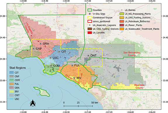
Figure 2. Study domain with name and three-letter code of the in-situ measurement sites used in this study. The SCI site is outside the inversion domain, and its measurements are only used to obtain background CH4 concentrations (location shown in figure S2). Average spatio-temporal area of dominance (STAD) for eight sites from February 2015 to May 2019 are color coded and the background layer shows the location of CH4 emitting facilities in the LA basin as described in the Vista-LA (see Carranza et al 2018). The dashed yellow line shows the area constrained by the eight sites in the domain.
Download figure:
Standard image High-resolution imageWe perform our inversions at 0.03° spatial resolution (1826 grid cells) and four-day temporal resolution for the period spanning from 27 January 2015 to 3 June 2020. Our emissions assessment is confined to the area constrained by the observations highlighted by the yellow outline in figure 2. The basis for this demarcation is described in Yadav et al (2019). The period for obtaining emissions estimates in this study was determined by the simultaneous availability of the measurements and the Jacobian from a coupled Weather Research Forecasting -Stochastic Time Inverted Lagrangian Model. The output from the WRF model for the LA basin was validated against data obtained from the Aircraft Communications, Addressing, and Reporting System and 42 surface observation sites data (see Yadav et al 2019 for details).
The location of the in-situ sites measuring surface CH4 concentrations (see Verhulst et al 2017 for discussion on the measurement network and the precision and accuracy of measurements) used in this study is shown in figure 2, and the temporal duration of the measurements with data gaps is shown in figure S1. CH4 enhancements (shown at monthly temporal resolution in figure S2) in this study are computed by subtracting the CH4 concentrations at the SCI site from those at the remaining sites using the methodology described in Verhulst et al (2017). This background site is located on San Clemente Island, which is outside the spatial domain of this study. Hourly temporal variability (standard deviation) of the CH4 concentrations and enhancements between 12:00 noon and 4:00 pm from 27 January 2015 until 22 April 2022 is used to assess trends in the temporal variability of CH4 concentrations. For inverse estimation of the CH4 emissions, we only use enhancements from 27 January 2015 to 3 June 2020 due to the reasons mentioned above.
3. Methods
We conducted a two-step analysis to fulfill the objectives of this study. First, we analyze the trend in the monthly temporal variability of the measured atmospheric CH4 concentrations rather than the concentrations themselves to detect the decline in CH4 emissions. In the second step, we quantify the magnitude of the reduction in CH4 emissions and confirm the evidence obtained from the previous mode of analysis through inverse modeling. The first step in our assessment is an exploratory approach to detect the change, and the second confirmatory approach relies on modeling to quantify emissions resulting from this change.
3.1. First step analysis: analysis of CH4 concentrations
For detecting changes in the CH4 emissions, we assume that temporal variability in CH4 concentrations is proportional to CH4 enhancements (for application, see Yadav et al 2021). We compute the monthly means of the hourly standard deviation of the CH4 concentrations processed at a cadence of 1 min. Following this, we fit a trendline (least squares regression line) to these time series and report the slope of these trendlines. We do not do this for the time series of CH4 enhancements as they contain large variability associated with weather conditions, making it difficult to isolate changes. In contrast, high-frequency (sub-hourly scale) variability is expected to directly correlate with emissions near the observation locations and be less affected by the synoptic conditions (see Umezawa et al 2020). However, for completeness, the time series of CH4 enhancements are also shown in figure S2. Note that this elementary exploratory analysis does not involve any models and relies only on measurements. Once we knew that the slopes of the trendlines were negative, we proceeded to do confirmatory analysis or modeling to estimate emissions.
3.2. Second step analysis: inverse estimation of emissions
Inversion forms the second step in our analysis. We use a geostatistical formulation of the atmospheric inverse problem to estimate CH4 emissions. The details of this approach within the context of the LA basin are covered in Yadav et al (2019), and a brief description is also given in section 1.1 of the supplementary material. The performance of inversions was assessed based on the metrics described by Yadav et al (2021). The results concerning this study are provided in the supplementary material in figure S5 of section 2.
We use the spatial-temporal area of dominance (STAD) metric based on atmospheric transport to spatially partition the LA basin. We did this to identify the regions where the most reduction in CH4 emissions happened during the time period of the study (figure 2). The mathematical details for identifying STAD regions are described in Yadav et al (2022), and a description is also provided in section 1.2 and figure S4 of the supplementary material. Note that our results only apply to the STAD areas, shown by the yellow outline in figure 2, which represents the study domain constrained by the observations.
4. Results and discussion
4.1. Assessment of the CH4 concentrations
We plot the mean monthly time series of the standard deviation of the CH4 concentrations in figure 3. The slope (units: parts per billion per month) of the trendlines computed after removing the data gaps for all time series is <0, indicating a reduction in CH4 emissions. However, compared to other sites, the pace of the decrease in the temporal variability was considerably higher for GRA and USC sites (see slopes in figure 3). For example, at the GRA site over 87 months (February 2015 to March 2022), this leads to a reduction in the temporal variability by 12.18 (−0.14 × 87 = −12.18; see equation in figure 3) parts per billion (ppb), which is about ∼1/2 of the peak temporal variability for 2021 (the last complete year for which data is available).

Figure 3. Monthly time series of the mean standard deviation of the CH4 concentrations for eight in-situ sites and for the combined concentration data from all sites titled 'All Towers'. A linear trendline (least squares regression line) for the time series of the standard deviation of the CH4 concentration and its equation and the standard error of the coefficients are also reported in the figure. We call the output from the equation 'Concvariability' which represents the variability in the concentrations, and 't', which represents a monthly time period. The slope in the equation is expressed in parts per billion per month. Note that we removed months for which data was not available to estimate the trendline.
Download figure:
Standard image High-resolution image4.2. Results: multiyear mean trend of CH4 emissions and uncertainties
To reduce the short-term noise and for understanding the long-term trend in the mean CH4 emissions, we plot seven four-day moving average of emissions (7 × 4 = 28 days) and uncertainties in figure 4. We chose this time period for averaging as it closely corresponds to the monthly duration of the assessment of the temporal variability of CH4 concentrations. However, all our results are based on unsmoothed time series of grid-scale emissions (submitted as a data record with this manuscript).
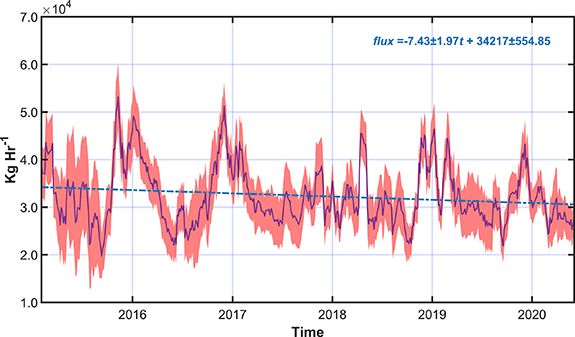
Figure 4. Time series of the inverse estimates of the mean four-day CH4 emissions for the LA basin with 1σ uncertainty. A linear trendline (least squares regression line) for the time series of CH4 emissions and its equation are also shown in the figure, as is the standard error of the coefficients. We call the output from the equation flux, where 't' represents a four-day time period. The slope in the equation is expressed in kg h−1 per four-day time period, and both the slope and intercept were significant with p < 0.01. Note the reduction in the seasonal amplitude (peak emissions-lowest emissions in a year) in the time series after 2017.
Download figure:
Standard image High-resolution imageThe trend in the four-day mean emissions confirms what was observed by assessing the temporal variability of CH4 concentrations. The average CH4 emissions declined by ∼2100 kg h−1 from February 2015 to May 2020 (figure 4). We can also partition the mean basin-scale emissions by STAD regions. Most of the basin is covered by the STADs of the ONT, FUL, GRA, and CIT sites. This applies both with respect to the area (figure 2) as well as prior emissions (figure S3).
Assessment of emissions by STADs shows that most of the reduction in emissions happened in the STADs of ONT and GRA (note the slope of the trendline in figure 5). Other STADs, except for these two, do not show any substantial changes in CH4 emissions. Due to the more extensive coverage of the STAD of ONT and GRA, the reduction of emissions in these regions had more significant impact on basin-scale CH4 emissions.
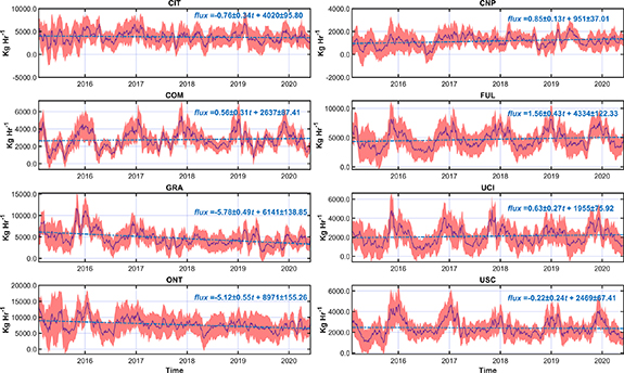
Figure 5. Time series of the inverse estimates of the mean four-day CH4 emissions for the STADs of eight in-situ sites with 1σ uncertainty bounds. A linear trendline (least squares regression line) for the time series of CH4 emissions and its equation are also shown in the figure, as is the standard error of the coefficients. We call the output from the equation 'flux', where 't' represents a four-day time period. The magnitude of the reduction or increase in the CH4 emissions can be determined from the slope of the equations expressed in kg h−1. The intercept for all sites was significant at p < 0.05, and the slope for all sites except COM and USC was significant at p < 0.05. Note the reduction in the seasonal amplitude in the time series of GRA and ONT sites after 2017.
Download figure:
Standard image High-resolution imageFigure 6 shows that the uncertainty on the estimated emissions declined over the time period of inversions; this is similar to the trend in the temporal variability of concentrations. This is consistent with a reduction in the seasonal amplitude (peak emissions minus lowest emissions in a year) of CH4 emissions, which can also be seen in figure 3 (see panel titled 'All Towers'), figures 4, and 5 for the STAD of ONT and GRA sites.
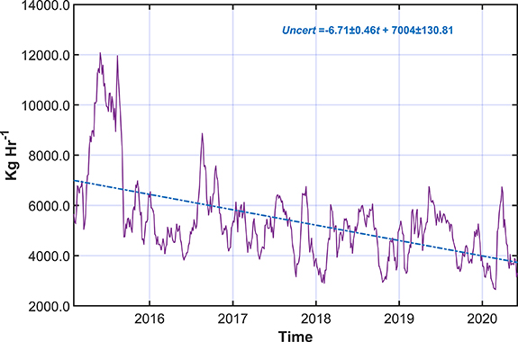
Figure 6. Time series of the uncertainty on mean four-day emissions estimated from inversions. A linear trendline (least squares regression line) for the time series with the standard error of the coefficients is also shown. The slope of the trendline is expressed in kg h−1, and both the slope and intercept were significant at p < 0.01. Note the reduction in the seasonal amplitude (peak uncertainty on emissions-lowest uncertainty on emissions in a year) in the time-series for the later years in comparison to the time period between 2015 and 2017.
Download figure:
Standard image High-resolution image4.3. Results: reduction in emissions for the LA basin at aggregated scales
We only report aggregated results for five years, from 2015 to 2019. Furthermore, as our inversions start from February 2015, we use the mean of the ratio of January emissions to the emissions for the remaining months in the years 2016–2019 to compute total CH4 emissions for January 2015.
Emissions at the annual scale declined in the basin from 2015. The difference between emissions for 2015 (272 ± 7.79 Gg; 1σ bound) and for years 2018 (244 ± 4.49 Gg; 1σ bound) and 2019 (251 ± 4.83 Gg; 1σ bound) was significant after accounting for >1σ uncertainty (figure 7). The emissions for 2018 and 2019 were significantly reduced even with respect to the emissions for 2017 (265 ± 5.03 Gg; 1σ bound). Emissions for 2018 were lower than those for 2019, though they were not outside each other's uncertainty bounds. However, emissions for 2018 were outside 2σ bounds with respect to 2016. For comparison, if we consider 2016 to be the baseline year as the last quarter of 2015 is influenced by the Aliso Canyon gas leak (duration: 18 October 2015 to 18 February 2016) then emissions of 2018 and 2019 were 10% and 7% lower, respectively. Note that emissions from the Aliso Canyon gas leak declined substantially from the start of the blowout on 23 October 2015, until 31 December 2015 (Conley et al 2016) and therefore, a comparison of 2018 and 2019 CH4 emissions with emissions for 2016 is unlikely to introduce any significant bias in the evaluation.

Figure 7. Total emissions for the inversion domain from 2015 to 2019 with 1σ uncertainty bounds. Note that we used the mean proportional emissions of January from 2016 to 2019 to get an estimate of emissions for January 2015.
Download figure:
Standard image High-resolution imageAssessment of the uncertainties themselves leads to an insight into the detectability limits of the network. Thus, with respect to 2016, a 7% annual reduction in the CH4 emissions in 2019 remains detectable at 1σ, whereas ∼10% reduction in 2018 was detectable at the 2σ level. In terms of magnitude, this difference of 10% corresponds to ∼800 kg h−1 or 11 Gg of CH4 emissions per year. To reiterate, a detection of 800 kg h−1 is applicable at an annual scale and not at an hourly temporal resolution.
At individual sites, we find declining emissions in the STADs of the GRA and ONT sites, but the rate of this decline is slowly plateauing (figure 8). These regions account for ∼45% of the emissions in the basin. The STADs for all other sites did not yield any significant trend in reduction (figure S6).

Figure 8. Total emissions with 1σ uncertainty bounds for the inversion domain for the STAD region covered by GRA and ONT in-situ site. Note that, like in figure 7, we used the mean proportional emissions of January from years 2016–2019 to get an estimate of emissions for January 2015.
Download figure:
Standard image High-resolution image
With respect to the 1σ uncertainty bound in figure 8, the emissions from STAD for GRA and ONT for 2018 and 2019 were significantly different from the baseline emissions for 2016. If we disregard 2015 as uncommon due to the Aliso Canyon gas leak, then differences between 2015 emissions from February to December and those for 2019 for ONT were significant after accounting for 2σ uncertainty bound on emissions.
4.3.1. Discussion: inverse estimates of emissions
The time series of the average emissions in figures 4 and 5 show a declining trend. However, if we look at the uncertainty bounds, then we cannot claim that the mean estimate of emissions for any four days is any different from emissions for other periods, and this is also applicable for the STAD regions. This implies that there has been no reduction in the four-day mean emissions estimate. However, average estimates of the emissions have the property of removing the impact of point sources. In comparison, aggregated emissions, as reported in figures 7 and 8, avoid this problem and provide a complete picture of the trend in emissions and their uncertainty, albeit at a lower temporal resolution. The CH4 emissions from the STAD for GRA and ONT significantly differed from the 2016 baseline emissions. Spatially, this is leading to a redistribution of CH4 emissions, whereby the overall contribution of the LA basin emissions from the STADs of GRA and ONT is declining, leading to an increase in the contribution from other STAD regions.
It can be argued that reductions in CH4 emissions are just an outcome of data gaps, atmospheric transport, or interannual variability. However, we do not think this is the case, as the trend in the suppression of the seasonal amplitude of the time series of mean emissions until May 2020 has been persistent for three years. This is also corroborated by the reduction in the temporal variability of CH4 concentrations, as shown in figure 3.
5. Conclusion
A higher bar consisting of multiple modes of analysis is required to confirm reductions in emissions from atmospheric observations, as the question is not only about estimating emissions but also about assessing the impact of policies implemented to reduce emissions. In this work, we show through our rigorous two-fold analysis that CH4 emissions in the LA basin are declining. However, the persistence of this trend has to be continuously monitored beyond the temporal duration of this study.
The inverse estimate of emissions and an exploratory analysis of the temporal variability showed that the seasonal amplitude of emissions has declined in the basin, leading to a reduction in annual CH4 emissions. However, identifying individual sources of these reductions from inversions with the existing measurement network is not directly possible.
Reasonable pointers to the sources that led to the emissions reductions can be obtained by analyzing (a) the nature of the sources of emissions and (b) the regions where this reduction has happened. Indeed, a consistent reduction in the seasonal amplitude of the temporal variability in concentration and emissions can most likely only be achieved by reducing fugitive emissions, a source of which is natural gas infrastructure in the LA basin (He et al 2019). Spatially, most of the reduction in CH4 emissions happened in the STAD regions of GRA and ONT that are dominated by CH4 emitting infrastructure consisting of landfills, dairies, and wastewater treatment plants. The GRA STAD covers the Sunshine Canyon Landfill, the largest landfill in the LA basin, and its emissions have declined due to improved management practices (see Cusworth et al 2020). We can disregard dairies as potential sources of emissions reduction, as they are only responsible for minimal or zero CH4 emissions in the LA basin (see Hsu et al 2010). We can also disregard wastewater treatment plants as sources of emissions reduction as they do not have a seasonal cycle of emissions whose amplitude can be reduced (see Daelman et al 2012 for variations in the CH4 emissions from a wastewater treatment plant). As a result, landfills and natural gas infrastructure are the most likely plausible sources of emissions reductions in the LA basin after 2015.
Finally, this study also shows that the existing network of surface measurements of CH4 concentrations in the LA basin can detect a 7%–10% reduction in CH4 emissions on an annual scale. However, identifying significant changes (outside the uncertainty bounds) in the mean emissions estimate will require assessment over a decade or more. We think that the availability of more observations could reduce this period; however, we do not explore this in the current study. In the near term, the research should focus on identifying individual facilities (e.g. landfills) responsible for CH4 emissions. This can help policymakers improve their oversight of the mitigation efforts undertaken by facilities to reduce CH4 emissions.
© Jet Propulsion Laboratory, California Institute of Technology.
Acknowledgments
A portion of the research described in this paper was carried out at the Jet Propulsion Laboratory, California Institute of Technology, under contract 80NM0018D0004 with the National Aeronautics and Space Administration (NASA). Additional support was provided by the National Institute of Standards and Technology (NIST) Greenhouse Gas and Climate Science Measurements program. The authors also acknowledge support from NASA's Carbon Monitoring System program and the Prototype Methane Monitoring System for California project and Multi-tiered Carbon Monitoring System project. Certain commercial equipment, instruments, or materials are identified in this paper to specify the experimental procedure adequately. Such identification is not intended to imply recommendation or endorsement by the National Institute of Standards and Technology, nor is it intended to imply that the materials or equipment identified are necessarily the best available for the purpose.
Data availability statement
Methane concentration data utilized in this study is already available from https://data.nist.gov/od/id/mds2-2388. This concentration data has also been submitted as part of this manuscript. Output of Weather Research and Forecasting and Stochastic Time-Inverted Lagrangian Transport Model is ∼50 terabytes in size and researchers interested in obtaining this data should provide authors a data repository to upload the model output.
Conflict of interest
The authors declare no potential conflicts of interest with respect to the research, authorship, and/or publication of this article.
Supplementary data (12. MB XLSX)
Supplementary data (1.6 MB DOCX)