
Abstract
Quantifying impacts of ecological disturbance on ecosystem carbon and water fluxes will improve predictive understanding of biosphere—atmosphere feedbacks. Tree mortality caused by mountain pine bark beetles (Dendroctonus ponderosae) is hypothesized to decrease photosynthesis and water flux to the atmosphere while increasing respiration at a rate proportional to mortality. This work uses data from an eddy-covariance flux tower in a bark beetle infested lodgepole pine (Pinus contorta) forest to test ecosystem responses during the outbreak. Analyses were conducted on components of carbon (C) and water fluxes in response to disturbance and environmental factors (solar radiation, soil water content and vapor pressure deficit). Maximum CO2 uptake did not change as tree basal area mortality increased from 30 to 78% over three years of beetle disturbance. Growing season evapotranspiration varied among years while ecosystem water use efficiency (the ratio of net CO2 uptake to water vapor loss) did not change. Between 2009 and 2011, canopy water conductance increased from 98.6 to 151.7 mmol H2O m−2 s−1. Ecosystem light use efficiency of photosynthesis increased, with quantum yield increasing by 16% during the outbreak as light increased below the mature tree canopy and illuminated remaining vegetation more. Overall net ecosystem productivity was correlated with water flux and hence water availability. Average weekly ecosystem respiration, derived from light response curves and standard Ameriflux protocols for CO2 flux partitioning into respiration and gross ecosystem productivity, did not change as mortality increased. Separate effects of increased respiration and photosynthesis efficiency largely canceled one another out, presumably due to increased diffuse light in the canopy and soil organic matter decomposition resulting in no change in net CO2 exchange. These results agree with an emerging consensus in the literature demonstrating CO2 and H2O dynamics following large scale disturbance events are dependent not only on tree mortality but also on the remaining and new vegetation responses because mortality and recovery occur at the same time.

Content from this work may be used under the terms of the Creative Commons Attribution 3.0 licence. Any further distribution of this work must maintain attribution to the author(s) and the title of the work, journal citation and DOI.
1. Introduction
Biosphere carbon (C) cycling is highly dynamic and tightly coupled with global climate change (Cao and Woodward 1998). Understanding controls of the C cycle within the biosphere is vital to constraining uncertainty and improving predictive understanding of ecosystem responses to disturbance (Kurz et al 2008b, Liu et al 2011). Globally, forests account for up to 80% of terrestrial aboveground C and ∼40% of belowground C (Dixon et al 1994, Roy et al 2001). Changes in factors regulating the C cycle have large global C implications, especially when potential positive feedbacks to climate change are considered (Dale et al 2001).
Forests in the US and Canada have 2–3% areal disturbance rates per year, primarily due to harvest and forest fire (Masek et al 2008). Harvest and fire disturbance impacts on ecosystems have been widely studied, including mechanisms controlling water quality (Carignan et al 2000), nitrogen cycling (DeLuca and Zouhar 2000) and net C cycling (Gough et al 2007). The mountain pine bark beetle (Dendroctonus ponderosae) infestation in the United States and Canadian Rockies is larger than any previously recorded outbreak (Kurz et al 2008a, Raffa et al 2008). Bark beetle impacts on ecosystem mechanisms may be similar to other disturbances (Ayres and Lombardero 2000, Hicke et al 2012). These include predicted reduction in plant CO2 uptake, increase in decomposition rates, decreasing leaf area and stem density (Edburg et al 2012), and changes to the water cycle (Mikkelson et al 2013). Ecosystem responses are also expected to be complex and variable both in space and time, owing to patchy vegetation dynamics during the mortality event with succession happen simultaneously (Rhoades et al 2013).
In temperate ecosystems, CO2 fluxes are primarily controlled by water availability (Pastor and Post 1986). Lack of available water can limit CO2 uptake below maximum potential of a given leaf area during dry years (Law et al 2002). When mountain pine beetles first appear, their attack affects water use of individual trees as they and their symbiotic blue-stain fungi reduce transpiration in infected trees (Edburg et al 2012, Yamaoka et al 1990, Hubbard et al 2013). Reduced transpiration from infected trees has been shown to alter water cycling processes, increasing soil moisture and drainage at the stand scale (Mikkelson et al 2013), and impacting snowpack dynamics (Biederman et al 2014, Pugh and Small 2012) and runoff (Bearup et al 2014). Water cycling changes are also expected to alter C cycling (Brown et al 2010, Brown et al 2012).
Carbon and water cycling are inherently linked through stomatal conductance within leaves by the transpirational loss of water while photosynthesis assimilates atmospheric CO2 (Katul et al 2009, Cowan and Farquhar 1977). Variation in ecosystem water use efficiency (WUE), defined as the ratio of ecosystem C gain to evapotranspiration (ET), is primarily linked to water availability of forested ecosystems (Ponton et al 2006). WUE is dependent on species present as well as canopy structure in the ecosystem (Monson et al 2010). Ecosystem canopy conductance, derived from ET measurements, can indicate decoupling of the C and water cycles (Granier et al 2000). For example, decoupling could occur in response to disturbance if canopy transpiration is reduced more than photosynthesis, or if water loss from soil evaporation increases under a more open canopy. Thus, changes in WUE may be a useful indicator of disturbance effects on ecosystem processes.
Mountain pine beetle disturbances are expected to release soil C to the atmosphere over long time scales due to increases in the decay of soil C pools coupled in the short term with reduced photosynthetic uptake (Goetz et al 2012, Edburg et al 2012, Harmon et al 2011, Hicke et al 2012). The net effect of both processes reduces net ecosystem productivity (NEP). However, it has been shown that tree mortality associated with disturbance can increase soil water availability (Mikkelson et al 2013), potentially increasing CO2 uptake in surviving trees (Law et al 2002). Increasing CO2 uptake from surviving trees can balance photosynthesis reduction from disturbance (Gough et al 2013). If evaporation does not increase enough to compensate for reduced transpiration due to bark beetle infestation (Hubbard et al 2013), ET from the ecosystem should decline (Mikkelson et al 2013). By monitoring NEP, ET, WUE and canopy conductance during the course of an outbreak, the changing controls of C and water cycling can be characterized separately from the effects of wet or dry years.
Review papers by Edburg et al (2012) and Mikkelson et al (2013) highlight expected changes to bark beetle impacted ecosystems. These include canopy mortality and soil water increases, both of which have cascading impacts on carbon and water cycles. The mechanism causing mortality by bark beetle infestation is similar to that of extreme drought stress (Yamaoka et al 1990, McDowell et al 2008). Therefore, we expect soil water content and ET responses to be similar to those of drought. Carbon cycling, as a balance of photosynthesis and respiration, will be controlled largely by different time scales of mortality, needle fall, and litter decomposition (Edburg et al 2012). To quantify ecosystem CO2 and water fluxes following a mountain pine beetle outbreak, we examined eddy-covariance data over three growing seasons as mortality increased within the tower footprint. We hypothesized that (1) bark beetle caused mortality will increase radiation and soil moisture while decreasing water flux to the atmosphere, (2) ecosystem WUE and canopy conductance will decrease as mortality increases during the course of the outbreak, (3) a decrease in photosynthesis and increase in respiration will cause net CO2 uptake to decline throughout the duration of the outbreak.
2. Methods
2.1. Site description
The study site is located in the Medicine Bow Range in Southeast Wyoming, near Chimney Park (41.37N 106.53W) at 2770 m elevation. The forest is primarily even aged with the last stand replacing fire 135 years ago and is composed of lodgepole pine (Pinus contorta, 81.2% basal area of study site), aspen (Populus tremuloides, 11.2%), and Engelmann spruce (Picea engelmannii, 0.8%). The area of the lodgepole pine forest vegetation extended 3 km in all directions from the eddy covariance tower. Mountain pine beetles (D. ponderosae) and the associated symbiotic blue-stain fungi (Grosmannia clavigera) were first observed at the site in summer 2007 and mortality within the study site was up to 79% in 2011.
Mean annual temperature of all three years at the site was 6.1 °C and monthly mean temperatures ranged from −7.3 °C (January) to 14.6 °C (August). The majority of precipitation falls during the winter months as snow. Maximum snow pack accumulations reached a snow water equivalent of 27.8 cm in 2010 and 28.4 cm in 2011, based on winter surveys done approximately one week before the snow pack turned isothermal (Biederman et al 2014). Snow melt generally occurs near the first week of May (Biederman et al 2014), and is associated with fully saturated soil and overland flow.
Average canopy height varied between 8.7 m and 16.2 m and the overall slope of the study area was under 2%. The longitudinal extent of the tower footprint was calculated based on average wind speed, average friction velocity, sensor height, zero plane displacement height and roughness length (Schuepp et al 1990). The tower footprint had a maximum straight line distance of 875 m to the west and 200 m to both the north and south, well within the extent of the forest study area. More than 95% of the average 30 min wind direction values were from the west.
2.2. Eddy covariance and environmental instrumentation
Above-canopy half-hour eddy-covariance measurements of water vapor flux (ET), sensible heat flux and CO2 flux began at the field site in January 2009. The eddy-covariance tower (18 m) was equipped with an open-path infrared gas analyzer (17.7 m) (LI-7500; LI-COR, USA), a sonic anemometer (17.7 m) (CSAT3; Campbell Scientific, USA), a four-component net radiometer (CNR1; Kipp & Zonen, the Netherlands) (17.1 m), and temperature and relative humidity sensors (HMP45C; Vaisala, Finland) (17.7 m and 3.7 m). Diffuse and direct photosynthetically active radiation at the top of the canopy was estimated based on Spitters (1986), using location of the field site and time of year. Transfer of radiation through the canopy was modeled based on Nijssen and Lettenmaier (1999), with an attenuation coefficient of 0.8 for both radiation types that is typical for pine canopies (Gower et al 1999). Soil moisture probes (CS616; Campbell Scientific, USA) were installed at 0–15 and 15–45 cm soil depths while two soil heat flux plates (HFP01SC; Hukseflux, Netherlands) were installed at a depth of 5 cm. Previous work at this study site (Parsons et al 1994) showed that >90% of roots are found within 40 cm of the surface, so both depths of soil moisture probes were averaged into one value based on weighted lengths of the probes. Growing season was defined as May 1st through October 1st and coincides with the average snow-free time period. Instruments for eddy covariance measurements were recorded at 10 Hz while all other sensors were recorded as half-hourly averages with a digital data logger (CR5000 or CR1000; Campbell Scientific, USA).
Ecosystem flux data were processed using MATLAB (2010a, The MathWorks) in the manner described in Lee et al (2004) including de-spiking the raw time series (Dale et al 2001) (Matlab code is contained as an appendix), addressing calibration drifts (Loescher et al 2009), coordinate rotation and planar fitting (Finnigan et al 2003), correcting for the time lag due to spatially separate sensors (Horst and Lenschow 2009), spectral corrections (Horst 2000, Massman 2000) and finally the WPL correction (Webb et al 1980). A friction velocity threshold of 0.089 m s−1 was established to screen out data based on Gu et al (2005), which included normalizing at diurnal and seasonal scales night-time CO2 fluxes using temperature response functions described in Gu et al (2002). All data with a friction velocity below this threshold were removed from our analysis, which accounted for only 1.4% of the total.
2.3. Canopy conductance
The Penman–Monteith equation was rearranged to give an expression for the ecosystem canopy conductance (Brümmer et al 2012).

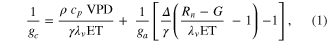
where Δ is the rate of change of the saturation specific humidity with air temperature, is dry air density, is the specific heat capacity of dry air, is the psychrometric constant, is the latent heat of vaporization and is the aerodynamic (boundary layer) conductance. , , and are measured net radiation, soil heat flux and vapor pressure deficit (VPD), respectively, from the site. A top-down ecosystem canopy conductance approach (Baldocchi et al 1991) was applied (Baldocchi et al 1987) that solved a nonlinear least squares curve fitting algorithm that fit both and at weekly time steps.


2.4. Light response curves
Ecosystem CO2 fluxo and radiation data were used to fit a Michaelis–Menten light response curve (Harley et al 1992, Falge et al 2001) to the data.

Solar radiation was used for the incoming radiation term, , to estimate quantum yield as the slope of the curve at low light levels and maximum assimilation as the asymptotic value at high light levels. Ecosystem respiration was estimated from curve fits using incoming solar radiation data. Curve fit parameters were calculated weekly over the course of the growing season in a manner similar to Zhang et al (2006). Weeks with less than 65% data coverage (Falge et al 2001) were discarded from this analysis.


Ecosystem respiration was also calculated with VPD limiting GEP, using light response curves and day-time data, following Lasslop et al (2010). was used to calculate gross ecosystem productivity (GEP) from NEE. Time series were gap-filled at the 30 min scale (Reichstein et al 2005) only for short gaps (less than one day) during the flux partitioning algorithm. Both GEP and values were averaged to daily time scales.


2.5. Water use efficiency
WUE on an ecosystem scale (eWUE) was defined as the slope of NEP to ET (VanLoocke et al 2012, Emmerich 2007), where positive NEP indicates uptake by the ecosystem. WUE was defined as the slope of GEP to ET (Law et al 2002); the values of eWUE will be somewhat smaller than WUE (Steduto and Albrizio 2005). Thirty minute fluxes were averaged on a weekly basis, again disregarding weeks with less than 65% of data. eWUE was calculated for each growing season as the mean of the weekly eWUE values following Law et al (2002) for WUE.
2.6. Scaling by leaf area index (LAI) and statistical analysis
The CO2 and water flux parameters of , ,, , , GEP, eWUE and WUE were normalized by yearly LAI values to convert parameters from a ground area basis to a leaf area basis. This was done to separate the yearly changes in the ecosystem parameters from the effect of a decline in the canopy leaf area. LAI measurements were taken once a year at 20 representative plots within the eddy-covariance footprint with a plant canopy analyzer (LAI-2000; LI-COR, USA). LAI was scaled to ecosystem level using a paint-by-numbers approach (Mackay et al 2002) that aggregated stand estimate of tree level basal area distributions data from 20 representative plots up to the ecosystem level of 144 plots. Four classes of tree basal area distributions were created that were similar to the four stands of trees measured for soil and tree temperature and moisture. Each of these four stands of trees were then considered representative of any of the 144 plots of the footprint that were most similar to them. Tree basal area and condition were measured annually in the 144 plots arrange along the tower footprint to track mortality due to beetle infestation. Basal area was used to estimate mortality at the footprint scale because basal area has been shown to be an appropriate scale for transpiration in ate lodgepole pine (Adelman et al 2008) and in other forest studies (Mackay et al 2010, Ford et al 2007). Autocorrelation of time series variables was addressed by computing differences between time steps of CO2 and ET fluxes while t-tests were used to statistically test for differences in parameters. MATLAB was used for all statistical and analytical work (MATLAB version 7.10.0. Natick, Massachusetts: The MathWorks, 2010).


3. Results
3.1. Controls of ecosystem fluxes
NEP (figure 1(a)) and ET (figure 1(b)) dynamics along with environmental controls of net radiation (figure 1(c)), VPD (figure 1(d)), and soil moisture (figure 1(e)) are shown against increasing site mortality, expressed as affected basal area percent (figure 1(f)). Site mortality expressed by density of trees was 38%, 55% and 68% in 2009, 2010 and 2011 respectively; lower than mortality by basal area due to bark beetle host selection favoring larger diameter trees. Net radiation and VPD were similar among years, but soil water content increased in 2010 and 2011. Snow melt began earlier in 2009 and full soil saturation was not observed during the growing season that year (Biederman et al 2014). In terms of snowpack, 2011 was a very wet year, and snow-water equivalent was estimated to be between 140% and 200% above the 30-year average from SNOTEL (Snowpack Telemetry) sites around the region. Despite the above-average snowpack in 2011, soil water content reached typical values by the end of the growing season. However, average ET was higher in the late growing season in 2011 than the other two years.

Figure 1. Seasonal variation in daily (24 h) average of (a) net ecosystem productivity at 17.7 m height, (b) ecosystem evapotranspiration flux at 17.7 m height, (c) net radiation at 17.1 m height with daily minimum and maximum values as shading, (d) mean vapor pressure deficit at 17.1 m height with minimum and maximum values as shading, (e) volumetric soil water content in the 0–0.45 m layer during the growing seasons of 2009–11 with tick labels relating to the 1st day of the month. Tree mortality percentage (of basal area) within the tower footprint by year for 2008–11 is shown in panel (f).
Download figure:
Standard image High-resolution imageRegression analyses of ET values showed weak and non-significant (p > 0.05) responses to soil moisture, net radiation, and vapor pressure deficit across the years of the study and regression slope coefficients between ET and soil moisture of all years are shown in table 1. Net radiation was a weak driver of ET in 2010. Regression coefficients for VPD were significant (p < 0.05) in 2010 and 2011, and as expected, an increase in VPD was linked to an increase in ET. The coefficients did not vary among years (p > 0.05).
Table 1. Regression slope coefficients for ET and canopy conductance as functions of environmental drivers (net radiation (Rn), vapor pressure deficit (VPD), soil moisture, and ET) for all three site years, excluding regression intercepts. Significant coefficients are in gray.
| Response | ||||||
|---|---|---|---|---|---|---|
| Predictor | ET 2009 (mg H2O m2 s−1) | ET 2010 (mg H2O m−2 s−1) | ET 2011 (mg H2O m−2 s−1) | Canopy Conductance 2009 (mmol m−2 s−1) | Canopy Conductance 2010 (mmol m−2 s−1) | Canopy Conductance 2011 (mmol m−2 s−1) |
| Rn (W m−2) | 0.00 | 0.01a | 0.00 | 0.07 | 0.45 | 0.12 |
| VPD (kPa) | 0.60 | 1.25b | 1.79b | −17.66 | 65.54a | 57.12 |
| Soil moisture | −1.18 | −0.78 | 4.42 | 398.64 | −9.78 | 3.80 |
| (%) | — | — | — | — | — | — |
3.2. Interannual variations in ecosystem WUE, canopy conductance and CO2 fluxes
Average NEP did not change among years even as tree mortality increased dramatically, with net CO2 uptake by the ecosystem remaining high throughout all three growing seasons (figures 1(a), 2(a)). Average values of of diffuse light increased in 2010 and 2011, as compared to 2009 (p < 0.05) (figures 2(b)–(d) and table 2). Ecosystem , and GEP did not change (p > 0.05) among years in this study (figures 2(e), (f)). While was generally smaller than , as expected due to high degree of VPD control over transpiration within lodgepole pine (Pataki et al 2000), both respiration estimates showed no differences between years (p > 0.05) as well.


Figure 2. Weekly averages of (a) net ecosystem productivity, (b) ecosystem respiration calculated from light response curves), (c) ecosystem respiration , including VPD limitation), (d) ecosystem quantum yield, (e), maximum ecosystem assimilation rates and (f) gross ecosystem production during the growing season for site years 2009–11.


Download figure:
Standard image High-resolution imageTable 2. Mean CO2 and water parameters for all three site years from the middle of the growing season (weeks eight through 15) with 95% confidence interval in parentheses.
| Year | Canopy conductance (mmol m−2 s−1) | Ecosystem respiration (μmol m−2 s−1) | VPD limited ecosystem respiration (μmol m−2 s−1) | Quantum yield (μmol m−2 s−1)/(W m−2) | Quantum yield of diffuse light (μmol m−2 s−1)/(diffuse W m−2) | Amax (μmole m−2 s−1) | eWUE With intercept not fixed at zero (μmol CO2 mg−1 H2O) | Intercept of eWUE (μmol CO2 m−2 s−1) |
|---|---|---|---|---|---|---|---|---|
| 2009 | 98.59 (14.10) | 2.00 (0.22) | 3.91 (1.08) | 0.054 (0.008) | 0.065 (0.002) | 19.6 (1.9) | 0.072 (0.06) | 2.32 (1.82) |
| 2010 | 145.38 (28.27) | 1.67 (0.30) | 2.96 (1.11) | 0.062 (0.012) | 0.066 (0.003) | 21.1 (3.4) | 0.061 (0.02) | 2.54 (0.72) |
| 2011 | 151.67 (25.72) | 1.60 (0.25) | 4.13 (0.87) | 0.064 (0.013) | 0.071 (0.002) | 19.8 (1.8) | 0.095 (0.04) | 1.46 (1.44) |
| Year | WUE With Intercept Not Fixed at Zero (μmol CO2 mg−1 H2O) | Intercept of WUE (μmol CO2 m−2 s−1) | NEP (μmol m−2 s−1) | GEP (μmol m−2 s−1) | — | — | — | — |
| 2009 | 0.113 (0.05) | 3.08 (1.53) | 2.78 (1.08) | 6.69 (0.68) | — | — | — | — |
| 2010 | 0.107 (0.05) | 2.51 (1.48) | 3.86 (1.11) | 6.82 (0.50) | — | — | — | — |
| 2011 | 0.117 (0.04) | 1.75 (1.42) | 3.18 (0.87) | 7.31 (0.45) | — | — | — | — |
Ecosystem increased in the middle of the growing season, compared to early season values (weeks 8–15) in both 2010 and 2011 (figure 3(a)). The growing season average in 2010 and 2011 both increased (p < 0.05) from 2009 (table 2).


Figure 3. Weekly averages of (a) ecosystem evapotranspiration flux and (b) ecosystem canopy conductance during the growing season for site years 2009–11.
Download figure:
Standard image High-resolution imageThe relationship between ecosystem and the driving variables soil moisture, net radiation, and VPD, showed no change among years (table 1). VPD was the only statistically significant predictor of in 2010 (p < 0.05) with a positive relationship between the variables. was not significantly related to net radiation or soil moisture.


eWUE and WUE showed no significant change among successive years (figure 4, table 2). All three study years had non-zero intercept terms for eWUE and WUE relationships between water and carbon dioxide. Ecosystem WUE measured at the same study area using gas exchange of shoots (Smith 1980) was 0.13 μmol CO2 mg−1 H2O, which was statistically comparable (p < 0.05) to our results in 2009 and 2011. Average water and CO2 fluxes from all three years of this study were lower than fluxes measured using the gas exchange method by Smith (1980) as expected when comparing whole forest canopies to fully illuminated shoots.

Figure 4. Weekly average water (ET) and CO2 (NEP) flux with fitted linear regression lines by year. Filled symbols are average ecosystem water use efficiency by year. Literature value from Smith (1980) is included.
Download figure:
Standard image High-resolution image3.3. LAI decline and ecosystem parameters
As mortality increased (figure 1(f)), LAI non-significantly (p > 0.05) declined from 2.16 in 2009 to 1.69 in 2011 while diffuse and direct solar radiation transfer through the canopy increased (table 3). Diffuse light at the top of the canopy made up 45% of the incoming solar radiation. Below canopy, both diffuse and direct light increased as a percentage of total incoming above canopy solar radiation. This increase in below canopy radiation was caused by the declining LAI.
Table 3. Values of measured LAI expressed in m2 of leaf area per m2 ground area, modeled below canopy diffuse light and below canopy direct light, expressed as a percentage of above canopy solar radiation.
| Year | Leaf area index (m2 m−2) | Below canopy diffuse light (%) | Below canopy direct light (%) |
|---|---|---|---|
| 2009 | 2.16 | 7.9% | 9.7% |
| 2010 | 1.94 | 9.6% | 11.6% |
| 2011 | 1.69 | 11.7% | 14.2% |
Effects of mortality-induced changes in canopy structure on ecosystem CO2 and water exchange were evaluated by normalizing growing season average , , , , , GEP, eWUE and WUE by LAI (table 4). The LAI-normalized values of , , and GEP were higher in 2011 than in 2009 (p < 0.05) and scaled of diffuse radiation increased every year (p < 0.05). Both and of diffuse radiation were not significantly different in 2009 and 2010 (table 2).


Table 4. Mean CO2 and water parameters normalized by LAI values for each year with 95% confidence interval in the mean in parenthesis.
| Year | LAI Normalized canopy conductance (mmol m−2 s−1) | LAI Normalized ecosystem respiration (μmol m−2 s−1) | LAI Normalized VPD limited ecosystem respiration (μmol m−2 s−1) | LAI Normalized quantum yield (μmol m−2 s−1)/(W m−2) | LAI Normalized quantum yield of diffuse light (μmol m−2 s−1)/(diffuse W m−2) | LAI Normalized Amax (μmole m−2 s−1) | LAI Normalized eWUE with intercept not fixed at zero (μmol CO2 mg−1 H2O) | LAI Normalized intercept of eWUE (μmole CO2 m−2 s−1) |
|---|---|---|---|---|---|---|---|---|
| 2009 | 45.64 (6.53) | 0.92 (0.10) | 1.81 (0.50) | 0.025 (0.004) | 0.030 (0.001) | 9.05 (0.86) | 0.033 (0.03) | 1.07 (0.84) |
| 2010 | 74.94 (14.57) | 0.85 (0.16) | 1.54 (0.57) | 0.032 (0.006) | 0.034 (0.002) | 10.86 (1.74) | 0.031 (0.01) | 1.31 (0.37) |
| 2011 | 89.75 (15.22) | 0.95 (0.15) | 2.44 (0.52) | 0.038 (0.008) | 0.042 (0.001) | 11.76 (1.04) | 0.056 (0.02) | 0.86 (0.85) |
| Year | LAI Normalized WUE with intercept not fixed at zero (μmol CO2 mg−1 H2O) | LAI Normalized intercept of WUE (μmole CO2 m−2 s−1) | LAI Normalized NEP (μmol m−2 s−1) | LAI Normalized GEP (μmol m−2 s−1) | — | — | — | — |
| 2009 | 0.052 (0.02) | 1.43 (0.71) | 1.29 (0.50) | 3.09 (0.31) | — | — | — | — |
| 2010 | 0.055 (0.02) | 1.29 (0.76) | 1.99 (0.57) | 3.51 (0.26) | — | — | — | — |
| 2011 | 0.069 (0.02) | 1.03 (0.84) | 1.89 (0.52) | 4.33 (0.27) | — | — | — | — |
4. Discussion
Results from this study show little change in the relationship between environmental drivers and fluxes during a major beetle outbreak, contrary to expectations. Water cycling within the ecosystem was complex, with eWUE not changing during the study while ecosystem and thus ET increased. Carbon cycling results were also not as expected, with , ,, and GEP all not changing, while only diffuse light increased.


During the course of the mountain pine beetle outbreak, the prediction that ecosystem photosynthesis would decrease (Edburg et al 2012) was not supported as the maximum assimilation parameter from the ecosystem light response curve and GEP from flux partitioning did not change and increased. While there is no pre-outbreak data from this study, the values found (19.6–21.1 μmole m−2 s−1) were similar to those in other temperate zone forests (Whitehead and Gower 2001). In a mixed northern hardwood forest girdling experimental treatment, CO2 uptake was sustained through similarly high canopy defoliation (Gough et al 2013).


Ecosystem parameter of diffuse light increased between 2010 and 2011. This is likely due to declines in LAI and canopy shading causing increased diffuse light penetration in the canopy similar to that found in a spruce beetle epidemic (Dale et al 2001). Increases in diffuse light have been linked to higher ecosystem productivity in other work (Gu et al 2002). Once the change in LAI was incorporated, diffuse light increased from 2009 and 2010 as well. Seasonal patterns in can be explained by variations in temperature among different forest types (Zhang et al 2006). As temperature was not significantly different among years, the observed increase in and diffuse canopy light throughout the study period is likely to contribute to the consistent NEP despite increasing mortality between all three years, as suggested by Gough et al (2013). Diffuse light within the canopy has a large effect on stomatal conductance at the leaf and canopy level (Ewers et al 2007) and net CO2 uptake from an ecosystem (Law et al 2002, Gough et al 2013). This work suggests that diffuse light impacts can be extended to forest disturbances and future process modeling should incorporate canopy light attenuation models that explicitly handle diffuse light.


With LAI declining throughout the beetle outbreak, increased amounts of modeled diffuse and direct light below the canopy allow more efficient CO2 uptake throughout the canopy as well as in the understory (Gu et al 2002). However, the needle drop process by dead trees is delayed at least two years after bark beetle infestation (Edburg et al 2012) thus the decline in LAI is lagged relative to mortality. Further, there are differences in LAI that attenuates radiation and LAI that no longer contributes to gas exchange before it falls off the dead trees illustrating the difference between LAI measured by light attenuation and effective LAI. Lag in LAI decline would explain the change noted in in 2010 and 2011 rather than at the start of the 2008 infestation. Canopy light-C interaction is hypothesized to increase in magnitude as the canopy continues to open and is one mechanism contributing to sustained and CO2 uptake values despite the mortality, in opposition to hypothesis 3. This process is also shown in the results of Brown et al (2012), Bowler et al (2012), and Amiro et al (2010) wherein CO2 uptake recovery from insect disturbances happens much more quickly than previously anticipated, considering the high mortality rates. This could be partly because trees that survive the mortality event take advantage of the extra water and nutrients that occur as root gaps form (Parsons et al 1994) and remaining trees grow faster (Hubbard et al 2013). Our results show that the 20% surviving trees and rapidly growing understory of lodgepole pine forests is a key feature leading to forest NEP and ET resiliency after bark beetle disturbance as suggested by overall indicators of forest management resiliency, similar to sustainable timber harvest management (Burton 2010).


The responses of ecosystem respiration, from light response curves and flux partitioning, showed no change, similar to the results of Brown et al (2012). This is likely a result of increased heterotrophic respiration and soil C decay (Edburg et al 2012, Harmon et al 2011) compensating for decreased autotrophic respiration as infested trees die. However, increased autotrophic respiration from residual vegetation responding to the increased light, water and nutrient environment cannot be ruled out. Ecosystem respiration is a main determinant of C balance in forests (Valentini et al 2000) so the predicted potential switch from a net CO2 sink to a CO2 source from modeling studies (Kurz et al 2008a, Kurz et al 2008b) is not supported from this site.
When normalized by LAI, several increases in ecosystem parameters appeared between years, including , both and diffuse light , , and GEP. This suggests changes in ecosystem CO2 and water functions are linked to changing canopy area, similar to the gypsy moth defoliation results of Clark et al (2010). This LAI normalized ecosystem response could provide an additional perspective on the contribution of autotrophic processes to ecosystem respiration; changes in LAI should be considered as scalars of fluxes in future ecological disturbance studies.


In contrast to our expectation in hypothesis 2 and the work of Brown et al (2012), we found that both eWUE and WUE did not change with increasing mortality but were similar to values reported for shoots in an undisturbed, nearby forest (Smith 1980). Along with increased ecosystem , this suggests the water flux signal is still dominated by transpiration. However the ecosystem transpiration is likely to include an increased understory proportion and may not have transitioned to an increased evaporation to transpiration state. If eWUE or WUE had dropped, as we expected, that would suggest more evaporation from the ecosystem per unit of CO2 uptake. However, eWUE or WUE can also remain constant even under high water stress (Zhang and Marshall 1994); indeed spruce trees dying from blue-stain induced mortality from spruce beetles continue to photosynthesize while they inevitably die (Dale et al 2001).

When considering ecosystem water and CO2 fluxes, total ET is related to the current age of the forest (Amiro et al 2006, Goulden et al 2006, Zimmermann et al 2000) while eWUE and WUE are both a function of water availability and stand age (Krishnan et al 2009). Values of water and CO2 fluxes from saplings are likely higher than from either a mixed or single aged mature forest (Law et al 2001, Phillips et al 2002). While the overall (three-year average) CO2 flux at this site was 49% lower as compared to Smith (1980), it is likely due in large part to intrinsic difference between saplings and mature ecosystems. In general, the eWUE and ecosystem flux values for all three site years were not out of range compared to other evergreen conifer study sites from the FLUXNET (Law et al 2002) and European (Kuglitsch et al 2008) synthesis studies; furthermore the observed lack of response of C cycling to mortality was similar to other forest disturbance results (Gough et al 2013, Gough et al 2007).
ET was not controlled by the expected environmental drivers of net radiation, VPD and soil water content and hypothesis 1 is rejected. In healthy pine forests in the Rocky Mountains, ET has been shown to be strongly related to leaf water potential (Running 1980) which is likely controlled by soil water content and VPD (Fetcher 1976, Pataki et al 2000). Even though year to year environmental control of water flux did not change during this study, mortality levels were already high (>50%) when flux measurements started. It is possible that ET declines had occurred prior to the start of this study in 2009. However, the smaller than expected response in ET is supported by the work of Biederman et al 2014, where stream flow amounts and water isotopic data from the same watershed as this study confirms that ET fluxes do not decrease and even increase as mortality increases. The possibility that surviving trees and re-growth are compensating for high mortality has been proposed by Mikkelson et al (2013) and seen in Biederman et al (2014), Rhoades et al (2013), and Hubbard et al (2013). Our work is the first to examine eWUE after mountain pine beetle mortality and contributes to an emerging literature that mountain pine beetles do not have consistent, large ecosystem consequences to water and carbon cycling. Our work combined with other recent papers illustrates that ecosystem resilience to insect-fungi induced mortality must be incorporated into predictions of future forests.
5. Conclusion
This study quantified the impacts of tree mortality induced by an insect epidemic on water and CO2 cycling and can be used to better understand environmental controls of these fluxes during the course of a large disturbance. Ecosystem WUE did not significantly change during the outbreak and was comparable values from undisturbed forests. An increase in GEP was found between 2009 and 2011. Ecosystem respiration and the efficiency of ecosystem to uptake CO2 with light increased over the outbreak, and changes were primarily attributed to declining canopy leaf area. The interaction between ecosystem WUE and CO2 uptake in the near future will determine if the ecosystem will be net C source or sink.

As mortality levels off due to lack of suitable sized host trees for the beetles, understory dynamics are expected to play a much larger role in C balance as the ecosystem recovers from the disturbance. Healthy, undisturbed lodgepole pine forests are characterized by a lack of understory vegetation and dry soils. However, beetle-induced mortality increases understory light and soil water and nutrient availability through root gaps. This shift in forest characteristics increases the importance of sub-canopy processes in regulating ecosystem CO2 and water fluxes while emphasizing the need for such mechanisms to be included in process models of forest recovery after insect-induced mortality.
Acknowledgments
The authors thank two anonymous reviewers for the improvements to this work based on their comments, J Angstmann, C Rumsey, D King, and F Whitehouse for field assistance, J Frank for eddy covariance data processing advice, S Peckham for field site management as well as Yost R and Zippy P for small mammal deterrence at the field site. This work was funded by National Science Foundation, UW Agriculture Experiment Station, Wyoming Water Development Commission, the United States Geological Survey, and the Wyoming NASA Space Grant Consortium.