
Abstract
Overuse of surface water and an increasing reliance on nonrenewable groundwater resources have been reported over various regions of the world, casting significant doubt on the sustainable water supply and food production met by irrigation. To assess the limitations of global water resources, numerous indicators have been developed, but they rarely consider nonrenewable water use. In addition, surface water over-abstraction is rarely assessed in the context of human and environmental water needs. Here, we perform a transient assessment of global water use over the historical period 1960–2010 as well as the future projections of 2011–2099, using a newly developed indicator: the blue water sustainability index (BlWSI). The BlWSI incorporates both nonrenewable groundwater use and nonsustainable water use that compromises environmental flow requirements. Our results reveal an increasing trend of water consumed from nonsustainable surface water and groundwater resources over the historical period (∼30%), and this increase is projected to continue further towards the end of this century (∼40%). The global amount of nonsustainable water consumption has been increasing especially since the late 1990s, despite a wetter climate and increasing water availability during this period. The BlWSI is the first tool suitable for consistently evaluating the renewability and degradation of surface water and groundwater resources as a result of human water over-abstraction.
Export citation and abstract BibTeX RIS

Content from this work may be used under the terms of the Creative Commons Attribution 3.0 licence. Any further distribution of this work must maintain attribution to the author(s) and the title of the work, journal citation and DOI.
1. Introduction
The sustainable use of global water resources is a key issue to economic development and food production. However, in recent years various studies report overuse of surface water and groundwater resources worldwide (Falkenmark 1989, Postel et al 1996, Gleick 2003, 2010, Oki and Kanae 2006, Döll et al 2009, Rodell et al 2009, Kummu et al 2010, 2014, MacDonald 2010, Vörösmarty et al 2010, Wada et al 2010, Famiglietti et al 2011, Konikow 2011, Wisser et al 2010, Gleeson et al 2012, Pokhrel et al 2012, Voss et al 2013, Gleeson and Wada 2013, Schewe et al 2013). Notable examples include the shrunk Aral sea (Pala 2006, 2011), the Colorado and the Yellow river heavily regulated by human water use and associated reservoir operations (Gleick 2003), and dwindling groundwater resources over intensely irrigated regions such as the Ogallala aquifer (Scanlon et al 2012b), the California's Central Valley (Famiglietti et al 2011), the North China Plain (Cao et al 2013), Northwest India and Northeast Pakistan (Rodell et al 2009, Tiwari et al 2009), and the Tigris–Euphrates (Voss et al 2013). Recent studies (Konikow 2011, Döll et al 2012, Wada et al 2012) suggest an increasing reliance of human water use on nonrenewable groundwater resources worldwide, casting significant doubt on the sustainability of regional water supply and associated food production met by irrigation.
To assess the degree of human water use on global water resources, numerous indicators have been developed. As overuse of water resources emerged in various regions of the world, in the late 1980s Falkenmark (1989) pioneered the concept of water shortage using a threshold value to describe different degrees of water scarcity. This is one of the most commonly used indicators in existence and is so-called the water crowding index (Falkenmark 1989). This indicator defines population-driven physical shortage of water in relation to principal water requirements (Rockström et al 2009). Water shortage occurs when the number of people competing for a limited water resources (∼blue water), i.e. water crowding is 'high' (empirically found to be >600 cap Mm−3 yr−1), or inverted, per capita water availability is 'low' to meet principal water requirements (<1700 m3 cap−1 yr−1) (Falkenmark et al 1997). Beyond 1000 cap Mm−3 yr−1 (or inverted, 1000 m3 cap−1 yr−1) chronic water shortage occurs, generally indicating a limitation to economic development.
Since then, the water scarcity indicator has evolved from simply country's per-capita water needs into a more comprehensive, spatially-explicit and sector-specific index including agricultural (irrigation and livestock) and industrial water needs at a finer spatial resolution (e.g., 0.5° or ∼50 km × ∼50 km at the equator). In the 2000s, several major water stress indicators have been developed. Raskin et al (1997), Vörösmarty et al (2000b), Oki et al (2001), and Alcamo et al (2003) compared total blue water demands (agriculture, industry and households) to blue water availability (∼river discharge) to expresses how much of the available water is taken up by the demand. Water stress is linked to difficulties in water use due to accessibility or mobilization issues (e.g., water infrastructure, flow control, costs), and is often expressed by a 'use-to-availability ratio' ('withdrawal to availability ratio' or 'consumption to availability ratio'), where values higher than 0.4 denote 'high' water stress (Rockström et al 2009). Extreme water stress is considered to occur at a ratio above 0.8. Alcamo et al (1997, 2000) alternatively used a 'criticality ratio' comparing annual water withdrawals to water availability, while Arnell (1999) used the simple water use to resource ratio, calculated at the national scale. Klepper and van Drecht (1998) applied a 'water satisfaction ratio' at a river basin scale to assess water stress. Douglas et al (2006) used the similar concept called 'relative water stress index'. In general, a region is considered to experience water stress when the ratio is higher than 0.4 considering the sustainability of renewable water resources. To test the robustness of the threshold value, Alcamo et al (2000) carried out a sensitivity analysis in which they recomputed the area of river basins falling under the water stressed category assuming different thresholds values for this category. They set a threshold of water stress as variable between 0.2 and 0.6 instead of a constant value of 0.4, depending on regions. Their results showed the differences between variables and a constant value of 0.4 are insignificant, which may suggest the robustness of a threshold value of 0.4 in these water stress indicators. For completeness, we note that water scarcity is the general collective term when water is scarce for whatever reason (Rockström et al 2009). Different from those water stress indicators, Meigh et al (1999) developed the water availability index, taking the temporal variability of water availability into account. The index compares the monthly blue water availability to the monthly blue water demands of all sectors [(water availability – demands)/(water availability + demands)]. The index is normalized to the range −1 to +1, with the month being maximum deficit or minimum surplus taken as decisive. Hanasaki et al (2008) explored whether water demand is fulfilled on a subannual basis using the newly developed 'cumulative withdrawal to demand ratio'.
Despite their global acceptance, these indicators have same major shortcomings. First, the indicators consider only the renewable surface and groundwater resources, and pay little attention to nonrenewable groundwater use that is often prevalent in (semi-)arid regions. Second, environmental flow requirements are rarely incorporated in these indicators with few exceptions (e.g., Smakhtin et al 2004, Falkenmark et al 2007, Rockström et al 2009). Indicators that include spatially-explicit environmental flow requirements are even fewer (e.g., Gerten et al 2013, Pastor et al 2013). In many regions streamflow, in particular baseflow, provides a reliable source of water to the environment, supplying water to aquatic and terrestrial ecosystems including vegetation (e.g., forest) particularly during a low flow period (e.g., drought). Assessing water resources considering nonrenewable groundwater use and environmental flow requirements is critical for developing sustainable water management as policy goal and management plans, especially where and to what extent to focus limited management resources. Third, nonrenewable water use is rarely assessed in the context of future human water needs, while nonrenewable groundwater resources are the major source of regional food production over semi-arid regions (∼20%) (Falkenmark et al 2009, Hoff et al 2010, Siebert and Döll 2010, Wada et al 2012). The expansion of irrigated areas has been slowing down in many countries, yet global food demand has been increasing consistently as a result of a growing world population. This may lead to an increasing reliance of food production on nonrenewable water use in near future. Moreover, the focus on renewable blue water resources only underexposes the impacts of socio-economic and climate change on the sustainability of human water use. An index that can evaluate the transient behavior of nonsustainable water use in the context of human water needs is therefore needed.
To perform a comprehensive assessment of global water use, we introduce a new indicator: the blue water sustainability index (BlWSI). The BlWSI incorporates both nonrenewable groundwater use and nonsustainable water use that compromises environmental flow requirements. The indicator assesses the sustainability of human water consumption considering the renewability and degradation of surface water and groundwater resources as a result of human water over-abstraction. We apply this indicator globally at a spatial resolution of 0.5°, but aggregate it to meaningful spatial units of subbasin to basin scale. With the indicator, we assess the sustainability of human water consumption over the historical period 1960–2010 as well as the future projections for 2011–2099.
In section 2, the methods, model and data used are described. The results are presented in section 3, and discussion is presented and the conclusions are drawn in section 4.
2. Methods, model, and data
2.1. Definition of BlWSI
The BlWSI is calculated from consumptive blue water use (CBWU), nonrenewable groundwater abstraction (NRGWA), and surface water over-abstraction (SWOA). CBWU is the sum of agricultural (livestock and irrigation), industrial, and domestic water consumption. NRGWA is computed from the difference between groundwater abstraction (GWA), and natural groundwater recharge (GWRNat) and additional recharge from irrigation return flow (GWRIrr) over the semi-arid and arid climate zones (Wada et al 2010). SWOA defines the amount of environmental flow requirements or environmental streamflow (QEnv) that is not satisfied due to local surface water consumptive use, including flow degradation already occurring from upstream water consumptive use. QEnv is the quantity of surface water flow that needs to be present to sustain environment and aquatic ecosystems, which is most important during low flow conditions. Although QEnv is best determined by the degree and nature of their dependency on streamflow, such information is rarely observed directly, especially at the scale at which it is modeled in this study. Therefore we equate QEnv to Q90, i.e. the monthly streamflow that is exceeded 90% of the time, following the study of Smakhtin (2001) and Smakhtin et al (2004). We calculated Q90 under the pristine or natural conditions (considering no water use in river routing; see section 2.2.) and used this to identify the surface over-abstraction (Qout − QEnv) due to human water consumption. BlWSI is thus defined as


where QIn is the inflow to a grid cell (i) and QOut is the outflow from the grid cell. QOut is calculated from simulated streamflow (during the river routing) that may be reduced by upstream human water consumption from all sectors (households, industry and agriculture; see section 2.3). When in a grid cell the available streamflow is less than the water consumption (consumptive use), no streamflow returns. Otherwise, the streamflow in excess of the local water consumption is accumulated along the drainage network and passed to the next downstream grid cell as inflow. Thus, for a streamflow that passes through major irrigated regions, QOut is much lower than QIn due to local irrigation water consumption (i) (QOut = QIn − CBWU). We perform this operation at each grid cell, considering the impact of upstream water consumption on downstream flow. Note that to avoid regions with negligible water consumption to be considered as regions with large SWOA, we replaced Q90 or QEnv with QOut whenever and wherever applicable (e.g., regions with only livestock water consumption).
The BlWSI is a dimensionless quantity and ranges between 0 and 1, which essentially expresses the fraction of the CBWU that is met from nonsustainable water resources (all in volume per time such as km3 yr−1). SWOA denotes rather environmental streamflow degradation, which can be seen as a proxy for nonsustainable human (surface) water abstraction. The indicator can be applied at a grid scale (i) such as 0.5° spatial resolution or it can be aggregated over a larger spatial extent such as subbasin or basin. This can be calculated at a variety of temporal units including month and year, but it is preferable to use a unit of multi-year average (e.g., decades) since sustainability is rarely assessed at short time scales. It should be noted that this indicator addresses sustainability only in terms of water quantity, but does not account for water quality, e.g. water pollution that affects the amount of readily available water over a region. Therefore, the assessment presented here may be considered as a low end of human water use sustainability.
2.2. Model simulation of blue water resources
The global integrated hydrological and water resources model PCR-GLOBWB (Wada et al 2010, van Beek et al 2011, Wada et al 2014) was used to simulate the terrestrial water balance (water in soil, rivers, lakes, reservoirs and wetlands) at a 0.5° spatial resolution for the historical (1960–2010) and the future period (2011–2099). In brief, the model simulates for each grid cell and for each time step (daily) the water storage in two vertically stacked soil layers and an underlying groundwater layer. The model computes the water exchange between these layers, and between the top layer and the atmosphere. The third layer represents the deeper part of the soil and constitutes a groundwater reservoir fed by active recharge, which is explicitly parameterized with a linear reservoir model (Kraaijenhoff van de Leur 1958). GWRNat fed by net precipitation and additional recharge fed by irrigation water are simulated as the net flux from the lowest soil layer to the groundwater layer, i.e. deep percolation minus capillary rise at a daily time step (see supplementary data for further model descriptions, available at stacks.iop.org/ERL/9/104003/mmedia).
Simulated specific runoff from the two soil layers (direct runoff and interflow) and the underlying groundwater layer (base flow) is routed along the river network based on the Simulated Topological Networks (STN30) (Vörösmarty et al 2000a) using the method of characteristic distances (Wada et al 2014). The model also calculates sectoral water demand, surface water and GWA, water allocation, consumptive use and return flows (see section 2.3 for the calculation of human water use). Abstractions, allocation and return flows are fully integrated into the hydrological model on a time-step basis and thus directly influence storage and flows in soil, surface water and groundwater (De Graaf et al 2014, Wada et al 2014). A reservoir operation scheme is also implemented based on the newly available and extensive Global Reservoir and Dams Dataset (GRanD) (Lehner et al 2011), which is dynamically linked with the routing module. Reservoir release is simulated to satisfy local and downstream water demands (∼withdrawal). In case of no water demand, reservoir release is simulated as a function of minimum, maximum, and actual reservoir storage (Wada et al 2014).
The model was forced with daily fields of precipitation, reference (potential) evapotranspiration and temperature. For the period 1960–1978, precipitation and temperature were prescribed by the ERA40 re-analysis data (Uppala et al 2005). Over the same time period, prescribed reference evapotranspiration was calculated based on the Penman–Monteith equation according to the FAO guidelines (Allen et al 1998) with relevant climate fields (e.g., cloud cover, vapor pressure, wind speed) retrieved from the ERA40 re-analysis data. To extend our historical analysis to the year 2010, we forced the model by comparable daily climate fields taken from the ERA-Interim re-analysis data (Dee et al 2011). From the ERA-Interim dataset, we obtained daily fields of temperature and GPCP-corrected precipitation (GPCP: Global Precipitation Climatology Project; www.gewex.org/gpcp.html), and calculated reference evapotranspiration by the same method retrieving relevant climate fields. For future projections, the model was forced with daily fields of precipitation, reference (potential) evapotranspiration and temperature taken from five global climate models (GCMs) and one underlying emission scenario (here accounted for by using the representative concentration pathway or RCP; see tables 1 and 2). Here, we focus on the RCP 6.0 or the 'middle of the road' scenario, that represents a global warming target of ∼4 °C by the end of this century. The newly available CMIP5 climate projections were obtained through the framework of the inter-sectoral impact model intercomparison project (ISI-MIP; www.isi-mip.org/). The GCM climate forcing was bias-corrected on a grid-by-grid basis (0.5°) consistently across five GCMs available in the project (Hempel et al 2013). The resulting bias-corrected transient daily climate fields were used to force the model over the period 2011–2099 with a spin-up, reflecting a climate representative prior to the start of the simulation period. In total simulations of five GCMs were used in this study (table 1). The result of each GCM is treated equally and no weight is given to a particular GCM based on the performance. As a result, 5 (5 GCMs × 1 RCP) projections were produced (see supplement for bias-correction of climate forcing).
Table 1. GCMs (global climate models)1 and scenarios (representative concentration pathways) used in this study.
| GCM | RCP | Period | Organization |
|---|---|---|---|
| HadGEM2-ES | 2.6, 4.5, 6.0, 8.5 | 1971–2099 | Met Office Hadley Centre |
| IPSL-CM5A-LR | Institute Pierre-Simon Laplace | ||
| MIROC-ESM-CHEM | JAMSTEC, NIES, AORI (The University of Tokyo) | ||
| GFDL-ESM2M | NOAA Geophysical Fluid Dynamics Laboratory | ||
| NorESM1-M | Norwegian Climate Centre |
1GCMs were obtained from the newly available CMIP5 (Coupled Model Intercomparison Project Phase 5; http://cmip-pcmdi.llnl.gov/cmip5/).
Table 2. Overview of representative concentration pathways (RCPs) (van Vuuren et al 2011).
| RCP | Scenario1 |
|---|---|
| 8.5 | Rising radiative forcing pathway leading to 8.5 W m−2 (∼1370 ppm CO2 equivalent) by 2100 |
| 6.0 | Stabilization without overshoot pathway to 6 W m−2 (∼850 ppm CO2 equivalent) at stabilization after 2100. |
| 4.5 | Stabilization without overshoot pathway to 4.5 W m−2 (∼650 ppm CO2 equivalent) at stabilization after 2100 |
| 2.6 | Peak in radiative forcing at ∼3.1 W m−2 (∼490 ppm CO2 equivalent) before 2100 and then decline (the selected pathway declines to 2.6 W m−2 by 2100). |
1Radiative forcing values include the net effect of all anthropogenic greenhouse gases and other forcing agents.
2.3. Calculation of human water use
Over the period 1960–2099, daily human water demand, withdrawal and consumption (water withdrawal minus return flow) from livestock, irrigation, industrial and domestic sectors were estimated (Wada et al 2011a, 2013b, 2014) over the 0.5° global grid using the latest available historical data and future projections on socio-economic (e.g., population, gross domestic product, access to water), technological (e.g., energy consumption, electricity production) and agricultural (e.g., livestock densities, irrigated areas, crop-related data, irrigation efficiency) drivers (gridded data and country statistics). The water use calculation used in this study has been tested and extensively validated using available country water use statistics (countries ≈ 200) in earlier work (Wada et al 2011a, 2011b, 2014). Here, to be consistent with the model simulation of blue water (see section 2.2) and due to data availability, we focus on the RCP 6.0 or the 'middle of the road' scenario under shared socioeconomic pathways (SSP2) that is comparable to a business‐as‐usual case. The newly available socio-economic and technological projection data under SSP2 scenario were obtained through the ISI-MIP (www.isi-mip.org/).
We computed livestock water use by combining livestock densities (i.e. the number of livestock per grid cell) with their drinking water requirements. We downscaled the country statistics of the numbers of each livestock type (cattle, buffalo, sheep, goats, pigs and poultry) for 200 countries (FAOSTAT; http://faostat.fao.org/) to 0.5° from 1960 to 2010 by using the distribution of the gridded livestock densities of 2000 (Food and Agriculture Organization of the United Nations (FAO) 2007). The future growth of country livestock densities was estimated in proportion to future change in country population since the change in livestock densities and population show a strong correlation over the past period 1960–2010. We assumed that no return flow to the soil or river system occurs from the livestock sector (Alcamo et al 2003, Wada et al 2011a, 2011b). Irrigation water use was simulated with PCR-GLOBWB (Wada et al 2014). The historical growth of irrigated areas (1960–2010) is accounted for by using country-specific statistics of irrigated areas for ∼230 countries (FAOSTAT) and by downscaling these to 0.5° using the spatial distribution of the gridded irrigated areas from the MIRCA2000 data set (Portmann et al 2010). However, due to the lack of future projections of land use patterns, future expansion of irrigated areas is not considered, and hence irrigated areas remain constant at the present extent. A few studies provide the future increase in irrigated areas but their estimates are low for most parts of the world: 0.6% yr−1 by 2030 for developing countries with 75% of the global irrigated areas (Bruinsma 2003); from 2.87 in 2005 to 3.18 million km2 in 2050 (Turral et al 2011); global growth rates of only 0–0.18% yr−1 by 2050 and then they stabilizes (Millennium Ecosystem Assessment 2005). For the irrigation sector, return flow occurs to the soil layers as infiltration and to the groundwater layer as additional recharge. Domestic and industrial water withdrawals were calculated by multiplying sector‐specific water use intensities by sector‐related socio‐economic drivers (population, GDP, electricity production, energy consumption). Technological change rates per country were then approximated by energy consumption per unit electricity production, which accounts for sector-specific restructuring or improved water use efficiency (Wada et al 2011a). The future improvement in water use efficiency implicitly accounts for future water saving trends in domestic and industrial sectors (under SSP2 scenario), that can be expected to occur in many currently developing countries in Asia, South America, and Africa. Return flow from water that is withdrawn for the industrial and domestic sectors is assumed to occur to the river system on the same day (no retention due to waste water treatment). For both sectors, the amount of return flow is determined by recycling ratios developed per country on the basis of GDP and the level of economic development (Wada et al 2011b), i.e. high income (recycling ratio of 80%; 20% of water is actually consumed), middle income (65%; 35% of water is consumed), and low income economies (40%; 60% of water is consumed) (see supplement and Wada et al (2011b) for further descriptions of the calculation of return flow and limited validation exercise).
Daily desalinated water use taken from the FAO AQUASTAT database and the WRI EarthTrends (www.wri.org/project/earthtrends/) (global total ≈ 15 km3 yr−1) was downscaled onto a global coastal ribbon of ∼40 km based on gridded population intensities and subtracted from the estimated total water withdrawal and consumption as an additional source of water supply. Future desalinated water use is assumed to change in proportion to country population size due to a strong correlation between population increase and desalinated water use growth rate over the historical period (1960–2010) (see figure S1 for the validation exercise). This assumption generally works well for countries with emerging economies and high population growth (e.g., Saudi Arabia, UAE, Oman, and Kuwait), however, it is not easily applicable to developed countries where the population growth is much milder (e.g., USA and Italy) (see figure S1). Gridded GWA was estimated using country GWA rates for 2000 that were obtained primarily from the IGRAC GGIS data base (www.un-igrac.org/publications/104), but also from the WRI EarthTrends, Foster and Loucks (2006), and Shah (2005) to expand the spatial coverage. Since the availability of historical GWA data is limited, the country GWA rates are assumed to change in proportion to country total water withdrawal over the years (Wada et al 2010). A limited validation exercise of this assumption is given in Wada et al (2014) who found that the method generally produces comparable trends of GWA to reported trends over years based on the assessment of ∼20 countries where historical data is available. The country GWA rates were then distributed to 0.5° grid cells, wherever surface water availability (water in rivers, lakes, reservoirs, and wetlands) is insufficient to meet the total water withdrawal (water withdrawal in excess of surface water availability) as a proxy for the locations where groundwater is abstracted to satisfy the deficits over countries (Wada et al 2012). The global hydrological and water use model runs with a daily time step, but the assessment was performed per month for this study. Detailed methodologies and validation of estimated global water use are given in Wada et al (2011a, 2011b, 2014).
3. Results
3.1. Global distribution of human water use and the past and future trend in human water use
Global maps of estimated and projected human water consumption from agricultural, industrial, and domestic sectors for the year 2010 and for the year 2099 are shown in figure 1 and the past and projected trends of global human water use including GWA are given in figure 2. For 2010, estimated global human water consumption totals ∼2000 km3 yr−1. Intense water consumption occurs over India, Pakistan, China, USA, Mexico, southern Europe, North Iran, and Nile delta, where more than 90% of the global irrigated areas are present. Over the period 1960–2010, human water consumption increased more than two-fold (∼250%). All sectors exhibit rapid increases of water consumption, but the bulk of this increase is attributable to a drastic rise in irrigation water consumption for growing food production, which more than doubled from ∼650 to ∼1400 km3 yr−1 over the past 50 years. Industrial and domestic (households') water consumption respectively tripled from ∼100 to 300 km3 yr−1 and quintupled from ∼60 to ∼280 km3 yr−1 due to rapid population growth and increased standard of living. Over the period 1960–2010, GWA shows also a consistent increase and nearly tripled from ∼350 km3 yr−1 to ∼1000 km3 yr−1. By the end of this century (∼2099), human water consumption is projected to increase further over many parts of the world, but the increase is particularly intense (>100%) over Africa, Central, West, and South Asia, Western USA, Mexico, and Central South America. The rising water consumption is primarily driven by rapid population growth and higher industrial activities (higher electricity and energy use) over currently developing countries in these regions. A large increase in domestic and industrial water use is also obvious in the global trends as shown in figure 2. Domestic water consumption is projected to more than double from ∼280 to ∼600 km3 yr−1 by the end of this century, while the increase in industrial water consumption is expected to be slightly milder from ∼300 to ∼550 km3 yr−1. Future irrigation water consumption (ensemble mean) was simulated over the present irrigated areas and thus the change only reflects projected climate change, i.e. warming temperature and changing precipitation patterns. It shows a much lower increase from ∼1400 to ∼1600 (±∼200) km3 yr−1 over the same period. The increase in irrigation water consumption is primarily driven by rising regional temperature and associated higher evaporative demand. We note that increasing atmospheric CO2 concentration may have a beneficial effect on crop growth and crop transpiration, however, it remains uncertain whether the CO2-induced lower crop transpiration due to improved water use efficiency may be canceled out by higher crop transpiration as a result of simultaneously increased biomass. Thus, the CO2 effect simulating irrigated crop water use was not considered in this study. Global human water withdrawals increased from ∼1700 to ∼4000 km3 yr−1 over the historical period 1960–2010 and is projected to increase further to ∼6000 km3 yr−1 by the end of this century, while global human water consumption is expected to rise to ∼3000 km3 yr−1.

Figure 1. Global maps of estimated and projected total blue water consumption (million m3 yr−1) for (a) 2010 and (b) 2099. The relative change (%) from (a) to (b) is given in (c).
Download figure:
Standard image High-resolution image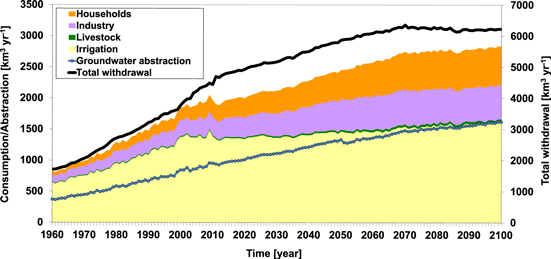
Figure 2. Estimated and projected trends of total blue water withdrawal (right y-coordinate), sectoral blue water consumption (households, industry, livestock and irrigation) and total groundwater abstraction (left y-coordinate) over the period 1960–2099 (km3 yr−1).
Download figure:
Standard image High-resolution image3.2. Subbasin analysis of BlWSI
Figure 3 shows maps of the long-term average BlWSI for surface water, groundwater and the two combined (total) calculated over the historical period (1960–2010). BlWSI was calculated at the subbasin scale to capture the spatial variability of nonsustainable human water use that occurs within a catchment. The indicator essentially signifies the fraction of human water consumption that is nonsustainable due to either environmental flow degradation or NRGWA (∼groundwater depletion), or both. Highest surface water over-abstraction is found over South, West, and Central Asia, Northeastern China, Spain, and Argentina where BlWSI (for surface water) exceeds 0.25, indicating that more than a quarter of surface water consumption is nonsustainable or sustained at the expense of environmental flow. BlWSI (for surface water) is also high over the western and central USA, Mexico, the Nile, and the Murray–Darling, where BlWSI corresponds to ∼0.1. For groundwater, BlWSI is close to or exceeds 0.5 over many regions including the Indus, Saudi Arabia, Iran, Algeria, the Southwestern and Central USA, and Northern Mexico. Over these regions, irrigation water consumption exceed 90% of the total and nearly or more than half of this consumption is sustained by NRGWA. These hotspots are also identified by recent studies that use satellite or ground-based observations (Rodell et al 2009, Tiwari et al 2009, Famiglietti et al 2011, Konikow, 2011, Scanlon et al 2012a, 2012b, Cao et al 2013, Voss et al 2013). Combining BlWSI for surface water and groundwater yields the total BlWSI. In particular, the Indus, Northeastern China, the Western and Central USA, Mexico, the Murray–Daring, and Southern Spain suffer from both surface and groundwater nonsustainable water use, aggravating the total BlWSI, whereas other regions tend to have a single source of nonsustainable water use.

Figure 3. Global maps of historical blue water sustainability indicator (BlWSI) (dimensionless) for (a) surface water, (b) groundwater, and (c) the total at a subbasin scale (except the Antarctica and Greenland) (1960–2010). The subbasin dataset was obtained from the FAO AQUASTAT database (www.fao.org/nr/water/aquastat/main/index.stm) that used the HydroSHEDS (http://worldwildlife.org/pages/hydrosheds) to derive the subbasins.
Download figure:
Standard image High-resolution imageFigure 4 shows same maps of the long-term average BlWSI for surface water, groundwater and the two combined (total) but now they are the ensemble mean of the five climate projections calculated over the future period (2069–2099). Figure 5 indicates the relative change of BlWSI for each water resource and the total from the historical to the future period. BlWSI is projected to worsen over most of the subbasins that are currently suffering from surface water over-abstraction and groundwater depletion. NRGWA will become more intense predominantly over (semi-)arid regions of the world, whereas surface water over-abstraction is projected to occur or be more severe over both arid and humid parts of the world including Europe, Southern China, Southern India and parts of Africa. The increase in (nonsustainable) surface water over-abstraction is driven by multiple factors: an increase in human water use (mainly from households, industry, or both sectors), a decrease in surface water availability, or higher low flow frequency (higher drought occurrence) such that environmental flow degradation is more susceptible to human water use. Adding to the current hotspot regions (e.g., the Indus and Northeastern China), future hotspots of nonsustainable water use from both surface water and groundwater appear over the southwestern USA, Mexico, Argentina, the Mediterranean region, the Middle East and Northern Africa region and Southern Africa. These regions will suffer from both increasing human water use and drier climate conditions by the end of this century. BlWSI exceeds 0.5 over many of these regions, where more than half of the human water consumption will likely be supplied at the expense of the degradation of environmental flow and the depletion of groundwater resources.
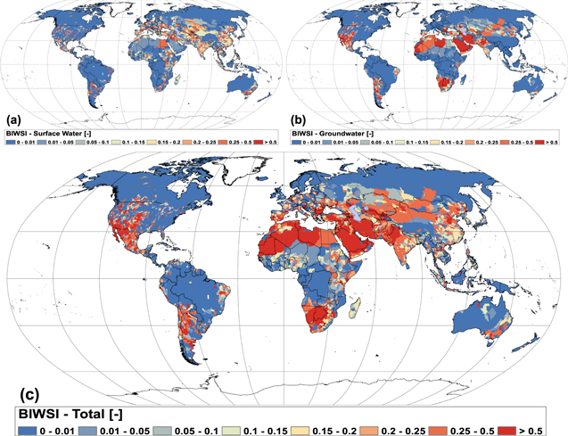
Figure 4. Global maps of future projected blue water sustainability indicator (BlWSI) (dimensionless) for (a) surface water, (b) groundwater, and (c) the total at a subbasin scale (except the Antarctica and Greenland) (2069–2099). The subbasin dataset was obtained from the FAO AQUASTAT database (www.fao.org/nr/water/aquastat/main/index.stm) that used the HydroSHEDS (http://worldwildlife.org/pages/hydrosheds) to derive the subbasins.
Download figure:
Standard image High-resolution image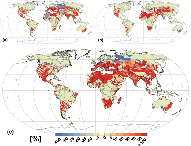
Figure 5. Relative change (%) of BlWSI for (a) surface water, (b) groundwater, and (c) the total at a subbasin scale from the historical (figure 3) to future period (figure 4) (except the Antarctica and Greenland).
Download figure:
Standard image High-resolution image3.3. Global trends in past and future nonsustainable water use and BlWSI
Figure 6 plots the estimated past trajectories and projected trends of surface water over-abstraction, NRGWA and the BlWSI at the global scale. The BlWSI shows a large inter-annual variability over the historical period, but afterwards this variability is partly filtered out due to the averaging of the five future projections (2011–2099). The BlWSI has been consistently increasing for the historical period 1960–2010 and is projected to rise even further by the end of this century. In 1960, ∼20% of the CBWU was supplied from nonsustainable water resources, with ∼80 km3 yr−1 and ∼90 km3 yr−1 from surface water over-abstraction and NRGWA respectively. In 2010, the share of nonsustainabile water consumption increased by ∼50% and became ∼30% of the total water consumption with ∼47% (∼270 km3 yr−1) and ∼53% (∼300 km3 yr−1) were met from surface water over-abstraction and NRGWA respectively. The increase has been evident particularly since the late 1990s when the share of nonsustainable water supply rose by ∼5% from ∼25% to ∼30% over merely a decade. During the 2000s, the warming temperatures raised the evaporative demand, which increased crop evapotranspiration and associated irrigation water demand. By the end of this century, the use of nonsutainable water resources is projected to increase to ∼1100 (±200) km3 yr−1, of which ∼45 (±10)% or ∼500 (±100) km3 yr−1 and ∼55 (±10)% or ∼600 (±100) km3 yr−1 will be met from surface water over-abstraction and NRGWA respectively. The global BlWSI is then expected to reach ∼0.4, indicating that ∼40% of the annual human water consumption will be nonsustainable.

Figure 6. Estimated trends of consumptive blue water use, surface water over-abstraction, nonrenewable groundwater abstraction (km3 yr−1) (left y-coordinate), and blue water sustainability indicator (BlWSI) (dimensionless) (right y-coordinate) over the period 1960–2099.
Download figure:
Standard image High-resolution image
Table 3 shows country estimates of total and NRGWA for major groundwater users. The share of nonrenewable to total GWA increased from ∼20% during the 1960s to ∼30% during the 2000s, indicating a growing reliance of human water use on nonrenewable groundwater resources. Over the period 1960–2010, a drastic increase of NRGWA is observed for India, Iran, and Saudi Arabia (a validation of groundwater depletion per region is given in Wada et al (2012)). The amount of NRGWA is projected to be doubled for almost all major groundwater users. The increase is particularly pronounced for India, Pakistan, USA and Mexico, where the regions with rising population and water use will coincide with those with decreasing surface water availability and groundwater recharge under climate change. For China, population growth is mild and climate change has a low impact on surface water availability and groundwater recharge. Over Iran and Saudi Arabia, the baseline surface water availability and groundwater recharge (for the historical period) is low and the increase in NRGWA will be driven by socio-economic change. For all major groundwater users, agriculture (∼irrigation) is often responsible for the largest part of the abstractions: India (89%), Pakistan (90%), Iran (90%), Saudi Arabia (90%) and Mexico (80%).
Table 3. Total and nonrenewable groundwater abstraction (km3 yr−1) over major groundwater users for 1960, 2010 and 2099.
| km3 yr−1 | Total (T) | Nonrenewable (N) | N/T (%) | (N)/(T) increase (%) | (T) per sector for 2010 (%) | |||||||||
|---|---|---|---|---|---|---|---|---|---|---|---|---|---|---|
| Country | 1960 | 2010 | 2099 | 1960 | 2010 | 2099 | 1960 | 2010 | 2099 | 1960–2010 | 2010–2099 | Agriculture | Domestic | Industry |
| India | 86 | 250 | 350 (±52) | 13 | 80 | 163 (±45) | 15 | 32 | 47 (±20) | 112 | 46 | 89.0 | 9.0 | 2.0 |
| USA | 57 | 125 | 137 (±28) | 9 | 23 | 56 (±12) | 16 | 18 | 41 (±18) | 17 | 127 | 62.0 | 20.0 | 18.0 |
| China | 52 | 110 | 169 (±42) | 8 | 28 | 36 (±8) | 15 | 25 | 21 (±10) | 65 | −15 | 74.0 | 12.0 | 14.0 |
| Pakistan | 38 | 80 | 108 (±21) | 22 | 46 | 75 (±24) | 58 | 58 | 69 (±25) | 0 | 20 | 90.0 | 8.0 | 2.0 |
| Iran | 34 | 72 | 98 (±18) | 18 | 47 | 65 (±11) | 53 | 65 | 66 (±24) | 23 | 2 | 90.0 | 6.0 | 4.0 |
| Mexico | 18 | 42 | 54 (±8) | 4 | 10 | 25 (±6) | 22 | 24 | 46 (±15) | 7 | 93 | 80.0 | 13.0 | 7.0 |
| Saudi Arabia | 4 | 25 | 42 (±6) | 3 | 20 | 32 (±8) | 75 | 80 | 76 (±25) | 7 | −5 | 90.0 | 10.0 | 0.0 |
| Globe | 372 | 952 | 1621 (±128) | 90 | 304 | 597 (±85) | 24 | 32 | 37 (±8) | 29 | 15 | 75.0 | 10.0 | 15.0 |
4. Discussion and conclusions
This study introduced the newly developed BlWSI. The BlWSI incorporates surface water over-abstraction and NRGWA to measure the sustainability of CBWU over the historical period (1960–2010) as well as the future projections (2011–2099). The global signal of BlWSI suggests an increasing trend of water supplied from nonsustainable water resources, where the global amount of surface water over-abstraction and NRGWA has been increasing especially since the late 1990s, despite larger water availability and higher evapotranspiration during this period as indicated by a recent study of Jung et al (2010). Nonsustainable water use typically occurs over (semi-)arid regions where the amount of precipitation is limited but the evaporative demand is high. Over these regions, groundwater pumping has been historically increasing to meet the demand (mostly for irrigation), resulting in an increasing reliance on depleting groundwater resources in recent years. Our future projections show that the situation is likely to continue as groundwater is a reliable source of water supply that can be used to meet the unmet water demands due to limited available surface freshwater. Readily accessible groundwater is an obvious choice to fill a gap between the increasing demands and limited availability of surface freshwater. However, the dependence on nonrenewable water resources likely increases the vulnerability of water supply as the degree of aquifer depletion is reported at an alarming rate over intensely irrigated regions including the Indus, Saudi Arabia, Iran, Northeastern China, the southwestern and Central USA, and Northern Mexico (Rodell et al 2009, Tiwari et al 2009, Famiglietti et al 2011, Konikow 2011, Scanlon et al 2012a, 2012b, Cao et al 2013, Voss et al 2013).
Previous studies of Vörösmarty et al (2005), Rost et al (2008), Wisser et al (2010), Hanasaki et al (2010), Wada et al (2010), Pokhrel et al (2012) and Yoshikawa et al (2013) quantified the amount of global NRGWA (some studies include the use of nonlocal water resources) (see table 4). These estimates range from ∼280 to ∼1200 km3 yr−1 for current conditions (∼2000). Our estimate of ∼250 km3 yr−1 (∼2000) lies in the lower range of these values. The main reason relates to the fact that most studies implicitly estimate the amount of NRGWA based on the amount of water demand exceeding locally accessible supplies of renewable blue water. Only Wada et al (2010) and this study use the information of GWA (both from IGRAC), which constrains the estimates. The estimates of the other studies are sensitive to both estimated water demand (1206–3557 km3 yr−1) and simulated surface freshwater availability (36 921–41 820 km3 yr−1). For the future, only Yoshikawa et al (2013) have provided an estimate of NRGWA to be ∼1150 km3 yr−1 (by 2050). Our estimate (∼450 km3 yr−1 by 2050) is less than half of their estimate primarily due to the reason described above and the large irrigated area expansion (from 2.7 in 2000 to 3.9 million km2 in 2050) considered in Yoshikawa et al (2013). They used globally a medium population growth scenario (0.9% yr−1) to extrapolate the future irrigated area change.
Table 4. Global estimates of nonrenewable groundwater abstraction.
| (km3 yr−1) | Total/Nonrenewable groundwater abstraction1 | Year | Withdrawal/Consumption | Runoff/Recharge | Sources |
|---|---|---|---|---|---|
| Data based estimates | |||||
| Postel (1999) | -/∼200 | Contemporary | — | — | Literature and country statistics |
| IGRAC-GGIS | ∼750/- | 2000 | — | — | Literature and country statistics |
| Shah (2005) | 800–1000/- | Contemporary | — | — | FAO AQUASTAT, Llamas et al (1992) |
| Zektser and Everett (2004) | 600–700/- | Contemporary | — | — | Country statistics |
| Model based estimates | |||||
| Vörösmarty et al (2005) | -/389Irr. -830Total | Avg. 1995–2000 | 3557Total-1206Irr. | 39 294/- | Simulated by WBM (0.5°) |
| Rost et al (2008) | -/730 | Avg. 1971–2000 | 2534–2566/1353–1375 | 36 921/- | Simulated by LPJmL (0.5°) |
| Döll (2009) | 1100/- | 2000 | 4020/1300 | 38 800/- | IGRAC-GGIS and WaterGAP (0.5°) |
| Wisser et al (2010) | 1708/1199 | Contemporary | 2997/- | 37 401/- | Simulated by WBMplus (0.5°) |
| Hanasaki et al (2010) | -/703 | Avg. 1985–1999 | -/1690 | 41 820/- | Simulated by H08 (1.0°) |
| Siebert et al (2010) | 545/- | 2000 | -/1277 | 39 549/12 600 | 15 038 national/sub-national statistics (irrigation) |
| Wada et al (2010) | 734(±82)/283(±40) | 2000 | -/- | 36 200/15 200 | IGRAC-GGIS and PCR-GLOBWB (0.5°) |
| Pokhrel et al (2012) | -/455(±42) | 2000 | 2462(±130)/1021(±55) | -/- | Simulated by MATSIRO (1.0°) |
| Döll et al (2012) | ∼1500/- | Avg. 1998–2002 | 4300/1400 | -/- | IGRAC-GGIS and WaterGAP (0.5°) |
| Yoshikawa et al (2013) | -/510 | 2000 | -/1358Irr. | -/- | Simulated by H08 (1.0°) |
| -/1150 | 2050 | -/2355Irr. | |||
| 372/90 | 1960 | 1708/828 | |||
| This study (2014) | 952/304 | 2010 | 4436/1970 | -/- | IGRAC-GGIS and PCR-GLOBWB (0.5°) |
| 1621(±128)/597(±85) | 2099 | 6223(±420)/2840(±280) | |||
1Some model based studies also include the estimate of nonlocal water abstraction (e.g., water supplied from cross-basin water diversions).
This study provides a comprehensive assessment of nonsustainable water consumption consistently across the globe. Note that Gosling et al (2010, 2011) and Haddeland et al (2011) indicate a large model-specific uncertainty using multi-model approaches. Our assessment involve two major sources of the uncertainty: human water use and blue water availability. Our methodologies to reconstruct past human water consumption follows the approach of Wada et al (2011a, 2011b, 2013a). In earlier work (Wada et al 2011a), the methods and outputs used in this study have been extensively validated using available country water use statistics (FAO AQUASTAT) and estimates (Shiklomanov 2000a, 2000b) for ∼200 countries, showing good agreement for most countries with R2 (the coefficient-of-determination) ranging from 0.91 to 0.97 and α (slope or regression coefficient) ranging from 0.94 to 1.16. However, it should be noted that large over- and underestimations (>30%) are also found for some countries over South America (Uruguay, El Salvador, Jamaica, Trinidad and Tobago, and Colombia) and Africa (Madagascar and Mali). Simulated blue water availability (water in rivers, lakes, wetlands, and reservoirs) and green water fluxes (∼actual evapotranspiration) have also been validated in earlier studies (van Beek et al 2011, Wada et al 2012). Simulated mean, minimum, maximum, and seasonal flow, and monthly actual evapotranspiration were evaluated against 3600 GRDC discharge observations (www.bafg.de/GRDC/) (R2 ≈ 0.9) and the ERA-40 reanalysis data respectively. We refer to van Beek et al (2011) and Wada et al (2012) for the details. In addition, simulated monthly total terrestrial water storage and low flow conditions (hydrological droughts) were evaluated and compared well with the GRACE satellite observations and GRDC discharge observations respectively for most of major catchments of the world (Wada et al 2012, 2013a). Yet, our assessment does not include any artificial water diversions, e.g. aqueducts, or inter-basin water transfer. Increasing water supply through water diversions tends to be a common response in water scarce regions with intense water use (Falkenmark and Molden, 2008). Such diversions can supply additional water to satisfy part of the nonsustainable water use. In some regions where extensive diversion works are present (e.g., India, USA, and China), our BlWSI assessment may therefore be somewhat overestimated.
Nonsustainable water use is a regional problem, but has both regional and global consequences, e.g. by depleting streamflow of transboundary (international) rivers or due to international food trade linking various nations across the globe. Once (nonsustainable) water resources are depleted or unavailable (e.g., economically or technologically unfeasible), irrigated crops relying on such resources will be severely impaired, which causes the loss of income for local farmers and a global decrease of crop production that may affect countries in another continent. To avoid such critical events to occur in the future, various measures have been proposed, involving innovations in water and food technology, water management and governance, dietary change, and economic incentives (e.g., environmental tax) (Gleick et al 2010, MacDonald 2010, Vörösmarty et al 2010, Fader et al 2010, 2013, Foley et al 2011, Kummu et al 2012). Water technology includes improving water recycling and irrigation efficiency (e.g., from sprinkler to drip irrigation) and recover losses (e.g., capture and use return flows in combination with partial purification). Innovations in food technology may involve the introduction of a variety of cultivars with higher water productivity (e.g., genetically engineered rice cultivars that are suitable without flood irrigation). However, these solutions require a substantial amount of economic investment that may not be easily realized for developing countries with limited financial and technological resources. The cultural dimension then may provide another solution such that a change in diet from rice to cereals (e.g., wheat and maize) would save a large amount of water that can then be used for other crops or other water use sectors. Water management and governance also plays an important role. For instance, subsidizing electricity or diesel fuel for groundwater pumps, in order to boost food production, leads to a large increase in active irrigation wells even in areas with available surface water and during the rainy season. Over such regions conjunctive use of groundwater and surface water resources can increase the water use efficiency and artificial recharge to aquifers (irrigation return flow) (Wada and Heinrich, 2013).
Our results reveal that ∼30% of the present human water consumption is supplied from nonsustainable water resources and this is projected to increase further to ∼40% by the end of this century (see table 4 for the comparison of NRGWA among different studies). It should, however, be noted that our estimates are rather optimistic since ongoing groundwater depletion may reach a critical point where groundwater level falls too deep or readily available groundwater resources are exhausted in regions currently suffering from severe depletion at some time during this century. The increasing degradation of environmental flows will pose a large threat to ecosystems around the world. Future population increase and economic development, therefore, cast significant doubt on future sustainability of human water use (Gleick, 2000, Alcamo et al 2003, Gerten et al 2011, Elliot et al 2013, Haddeland et al 2013). At the same time, our estimated degree of future nonsustainable water use may be underestimated since we did not consider the future expansion of irrigated areas, that will likely further rise the amount of human water use. Our future irrigation water use is ∼25% lower compared to that of Hanasaki et al (2013a, 2013b) and Yoshikawa et al (2013) (see table 5 for the comparison of future sectoral water use among different studies). However, the increase in irrigation intensity and water productivity, and the improvement in irrigation efficiency may substantially mitigate the rise in future irrigation water demand. For industrial and domestic sector, our future estimates are in line with those of Hanasaki et al (2013a, 2013b) and Yoshikawa et al (2013). In addition, climate change will bring more extreme climate conditions and higher low flow frequency in many parts of the world (Lehner et al 2006, Feyen and Dankers, 2009, Prudhomme et al 2013, Trenberth et al 2014), which will increase our reliance of water use on groundwater resources (Famiglietti et al 2011, Scanlon et al 2012a, 2012b). Although decreased surface water availability can be buffered by increasing reservoir release in regions where infrastructure (e.g., dams) is present (e.g., North America and Europe), there are many regions with low buffering capacities and the construction of new reservoirs has been generally slowing down. It is thus of critical importance to quantitatively assess how long the nonsustainable water use can keep up with the increase in human water use worldwide and to analyze sets of mitigation measures to help create a long-term sustainable, resilient water-food nexus. A vast amount of fossil groundwater reserves in the Nubian Aquifer System (the Nubian Sandstone Aquifer and the Post Nubian Aquifer System) will not dry up for coming decades (150 000 km3 stored and ∼100 km3 depleted over 1900–2008) (CEDARE 2001, Konikow 2011), however, reliable information of readily accessible groundwater reserves in many aquifers is largely unknown. The current degree of nonsustainable use may compromise the future livelihoods of millions of people and their living standards.
Table 5. Comparison of estimated sectoral water use (withdrawal and consumption) to other estimates.
| km3 yr−1 | Withdrawal/Consumption | 1960 | 2000 | 2025 | Mid-century (∼2050) | End-century (∼2090) |
|---|---|---|---|---|---|---|
| Agriculture (irrigation/livestock) | ||||||
| Hanasaki et al (2013a, b) | 3214/- | — | 4137/- | 4829/- | ||
| Yoshikawa et al (2013) | -/671 | -/1358 | — | -/2355 | — | |
| This study | 1278/655 | 2644/1392 | 3385/1422 | 3490/1494 | 3664/1655 | |
| Industry | ||||||
| Hanasaki et al (2013a, b) | — | — | 1169/- | 1437/- | 1259/- | |
| Yoshikawa et al (2013) | — | — | — | — | ||
| This study | 356/116 | 752/257 | 1084/348 | 1443/489 | 1438/551 | |
| Domestic | ||||||
| Hanasaki et al (2013a, b) | 598/- | 822/- | 973/- | |||
| Yoshikawa et al (2013) | — | — | — | — | — | |
| This study | 85/57 | 328/199 | 609/337 | 930/470 | 1116/623 | |
Acknowledgements
We cordially thank three anonymous referees for their constructive and thoughtful suggestions, which substantially helped to improve the quality of the manuscript. This work has been supported by the framework of ISI-MIP funded by the German Federal Ministry of Education and Research (BMBF) (Project funding reference number: 01LS1201A). Y W was financially supported by Research Focus Earth and Sustainability of Utrecht University (Project FM0906: Global Assessment of Water Resources) and the American Geophysical Union (AGU) Horton (Hydrology) Research Grant (2012). This research benefited greatly from the availability of invaluable data sets as acknowledged in the references.