
Abstract
Bacterial community structure and the effects of environmental factors on the microbial community distribution were investigated in the Changjiang Estuary hypoxia area and its adjacent area in the East China Sea (ECS) in June, August and October, 2006. Profiles of bacterial communities were generated by denaturing gradient gel electrophoresis (DGGE) of 16S rRNA genes followed by DNA sequence analysis. The dominant bacterial groups were affiliated to Gammaproteobacteria, Cytophaga–Flavobacteria–Bacteroides (CFB), Deltaproteobacteria, Cyanobacteria and Firmicutes, which were mostly from the marine seawater ecosystem. Effects of environmental factors on the bacterial community distribution were analyzed by the ordination technique of canonical correspondence analysis (CCA). The environmental factors significantly influencing bacterial community structure were different in the three months; dissolved organic carbon (DOC) and temperature in June and nitrite in August. No environmental variables displayed significant influence on the bacterial community at the 5% level in October. The seasonal environmental heterogeneity in the Changjiang Estuary and the adjacent ECS, such as seasonal hydrodynamic conditions and riverine input of nutrients, might be the reason for the difference in the key environmental factors determining the bacterial community in the three months.
Export citation and abstract BibTeX RIS
1. Introduction
Bacteria, as one of the members of the microbial food loop, play critical roles in nutrient cycling and energy flow in the marine ecosystem (Azam et al 1983, DeLong and Karl 2005). Knowledge of bacterial community composition is important for the understanding of the global patterns of marine bacterial diversity (Pommier et al 2007) and even for comprehension of local and global biogeochemical processes (Zehr and Ward 2002, DeLong and Karl 2005, Strom 2008).
Hypoxia has become a world-wide phenomenon in the global coastal ocean and causes a deterioration of the structure and function of ecosystems (Diaz and Rosenberg 2008, Kemp et al 2009, Rabalais et al 2010, Zhang et al 2010). Hypoxia also has a profound impact on ecosystems, such as the emission of greenhouse gases to the atmosphere (Bange et al 1996, Paulmier and Ruiz-Pino 2009), change in the food-web structure and system function (Bograd et al 2008, Stramma et al 2008, Middelburg and Levin 2009, Stramma et al 2010), and changes in organism life cycles (Fernández-Alamo and Färber-Lorda 2006, Paulmier and Ruiz-Pino 2009). A massive amount of research on hypoxia has been carried out in the global ocean (Zhang et al 2010), including the causes of hypoxia, biogeochemical processes in hypoxia, and the impact on the sustainability of the ecosystem. Microbiological studies in the hypoxia area mainly focus on bacterial and archeal community composition (Stevens and Ulloa 2008, Liu et al 2011), the vertical distribution and activity of anammox bacteria (Galán et al 2009), ammonia-oxidizing archeal community structure (Molina et al 2010) and communities of nirS/nirK-type denitrifiers (Liu etal 2003, Castro-González et al 2005). However, little is known about the relationship between environmental factors and microbial community structure in the hypoxia area.
The East China Sea (ECS) is a continental marginal sea of the western Pacific Ocean. The Changjiang Estuary, located offshore from the mouth of the Changjiang River, is an area where freshwater and Changjiang diluted water is mixed with the Taiwan Warm Current (TWC) from the south and Yellow Sea coastal water from the north (Chen et al 1999). Because it is an important interface between terrestrial and marine environments, this region is highly complex and dynamic (Zhang et al 1999). Therefore, the Changjiang Estuary and the adjacent ECS are ideal areas for ecological studies on temporal and spatial dynamics of biota. More interestingly, seasonal hypoxia in near-bottom waters occurs in the region off the Changjiang Estuary in summer (Li et al 2002, Zhu et al 2011). How the bacterial community responds to such changing conditions is very important for the understanding of structure and function of the estuarine ecosystem. Although a few bacterial community studies have been carried out in this area (Jiao et al 2005, Zhang and Jiao 2007, Feng et al 2009), little is known about the effects of hypoxia on the diversity and distribution of bacteria.
In this study, we examined the temporal distribution of the bacterial community in the Changjiang Estuary hypoxia area and its adjacent area in the ECS by denaturing gradient gel electrophoresis (DGGE) analysis. Additionally, the contribution of several environmental factors to bacterial community distribution was assessed using multivariate analysis techniques.
2. Materials and methods
2.1. Study sites and sample collection
Three cruises were conducted in June, August and October, 2006, respectively, in Changjiang Estuary hypoxia area and the adjacent East China Sea. Five stations (H32, H12, H15, H22 and H26) were chosen, with the former two stations in the hypoxia zone (figure 1). Hypoxia is defined as dissolved oxygen < 2 mg l−1 (Zhu et al 2011). Samples in June, August and October were named as H-1-, H-2- and H-3-, respectively. Three layers (surface, middle and bottom) were studied for every station. For every sample, 9 l seawater (for three replicates) for microbial diversity analysis were taken with Niskin bottles fixed on an SBE25 CTD (Sea-Bird Electronics).
Seawater was filtered onto 0.2 µm pore size, 47 mm polycarbonate filters (PFs) (Millipore) after pre-filtration through 3 µm pore size, 47 mm PFs. Filters (0.2 µm) for DNA extraction were then stored at −20 °C.
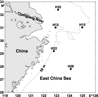
Figure 1. Map showing the five sampling stations.
Download figure:
Standard image2.2. Measurements of physicochemical parameters
For each sample, in situ measurements of the physicochemical parameters of seawater (depth, dissolved oxygen, pH, salinity and temperature) were recorded with the SBE25 CTD. Other parameters were measured in the laboratory. The Chl a concentration was determined fluorometrically using a Turner Designs fluorometer (provided by Chenggang Liu, Second Institute of Oceanography, State Oceanic Administration). Data on nitrate, nitrite, ammonium, silicate, phosphate, particulate organic carbon (POC) and dissolved organic carbon (DOC) were obtained from the State Key Laboratory of Estuarine and Coastal Research, East China Normal University.
2.3. DNA extraction
Genomic DNA was extracted and purified using lysozyme, proteinase K and sodium dodecyl sulfate with chloroform extraction and isopropanol precipitation, following Abell and Bowman (2005). DNA extractions from three replicates were pooled for each sample.
2.4. PCR amplification and DGGE analysis
The v3 region of the bacterial 16S rRNA gene was amplified from genomic DNA using bacterial-specific primers 341F-GC ( -3') and 534R (5'-ATTACCGCGGCTGCTGG-3') (Muyzer et al 1993).
The PCR was performed using the following program: 94 °C for 10 min; followed by 20 touchdown cycles of denaturation (at 94 °C for 1 min), annealing (at 65–55 °C for 1 min, decreasing 0.5 °C each cycle) and extension (at 72 °C for 1 min); 15 standard cycles of denaturation (at 94 °C for 1 min), annealing (at 55 °C for 1 min) and extension (at 72 °C for 1 min), and a final extension at 72 °C for 10 min. To reduce possible inter-sample PCR variation, all PCR reactions were run in triplicate and pooled together before loading on the DGGE gel. In PCR amplification, genomic DNA of E. coli was used as a positive control and PCR mixture without a DNA template was used as a negative control.
DGGE was performed using a Dcode™ Universal Mutation Detection System (Bio-Rad, USA). PCR products were separated on a vertical gel containing 8% polyacrylamide (acrylamide:bisacrylamide ratio of 37.5:1) and a linear gradient of the denaturants (urea and formamide), which increased from 40% at the top to 65% at the bottom of the gel. Electrophoresis was performed at 58 °C in a 1×TAE buffer at 65 V for 10 h. The gel was stained with SYBR Green I and DNA bands were visualized and photographed with a Canon A640 digital camera (Canon Co., Ltd, Japan).
2.5. Analysis of DGGE banding pattern
For sample comparison, DGGE band position and intensity in each gel track were determined using the Quantity One Program (Bio-Rad, USA). Lane background was subtracted by using a rolling disk size of 8 (Salles et al 2004, Zeng et al 2009). Band matching was performed with the tolerance and optimization setting at 1.00% (Salles et al 2004). Cluster analysis of the DGGE banding pattern was performed with the NTSYS pc-package (Rohlf 1988) using the unweighted pair group method with arithmetic mean (UPGMA), based on the presence or absence of each band (Abell and Bowman 2005).
2.6. Multivariate statistical analysis
The relationship between DGGE profiles and the seawater physicochemical properties was studied. To test whether weighted-averaging techniques or linear methods were appropriate, detrended correspondence analysis (DCA) was performed using CANOCO for Windows 4.5 (Biometris, Netherlands).
The longest gradients resulting from DCA were 1.652, 2.794 and 1.878 for the analysis based on DGGE profiles in June, August and October, respectively. These values did not indicate a clear linear or unimodal relationship (Lepš and Šmilauer 2003). We performed canonical correspondence analysis (CCA) to compare species–environment correlations.
An automated forward selection was used to analyze inter-sample distances for DGGE profiles. First, the variance inflation factor of environmental variables was calculated. Variables displaying a value greater than 20 of this factor were excluded from CCA analyses, assuming collinearity of the respective variable with other variables included in the examined dataset.
The analysis was performed without transformation of data and focus scaling on inter-sample distances. Manual selection of environmental variables, applying a partial Monte Carlo permutation test (499 permutations) with unrestricted permutation, was performed to investigate the statistical significance (Salles et al 2004, Sapp et al 2007). The marginal effects of environmental variables were selected according to their significance level (P < 0.05) prior to permutation. Ordination biplots including the environmental variables and DGGE samples (lanes) were used to explain our data.
2.7. Sequencing of DGGE bands and phylogenetic analysis
Strong and well-isolated DGGE bands were excised from the gel, washed with 500 µl sterile water three times and then DNA was eluted into 50 µl sterile water by incubation at 4 °C overnight. After centrifugation at 11 000g for 60 s, the supernatant was used as a template for the PCR-DGGE analysis to check for band position and purity. After that, DGGE bands were re-amplified with no GC clamp forward primer. PCR products were purified and cloned into a TA vector using pMD18-T (TaKaRa, Japan). The insertion of DNA fragments with appropriate sizes was confirmed by PCR amplification with M13-47 and RV-M primers, which corresponded to both sides of the cloning site on the vector. The 16S rRNA genes from DGGE were sequenced using the primer M13-47 or RV-M in the GenScript USA Inc. (Nanjing, China).
2.8. Nucleotide sequence accession numbers
Sequences from DGGE bands were submitted to the GenBank database with the accession numbers EF433 334–EF433 362, EF433 369–EF433 371 and EF467 882–EF467 884.
3. Results
3.1. Environmental characterization
Due to the influences of Changjiang River freshwater, the surface water at the H12 station had the lowest salinity but the highest concentration of Chl a, DOC and POC (table 1). Hypoxia was observed at stations H12 and 32 during sampling in August (table 1). In June, as a result of the intrusion of the cold water mass from the Yellow Sea (Zhao 1987), the temperature of sample H15-1-B was the lowest.
Table 1. Environmental data in June, August and October, respectively. (Note: Temp, temperature; Sal, salinity; DO, dissolved oxygen; DOC, dissolved organic carbon; POC, particulate organic carbon; -1, -2 and -3, samples collected in June, August and October, respectively; -S, -M, -B, samples collected from surface, middle and bottom layers, respectively.)
| Samples | Depth (m) | Temp (°C) | Sal | pH | DO (mg l−1) | Chl a(mg m−3) | DOC (µmol l−1) | POC (µmol l−1) | NO3− (µmol l−1) | NO2− (µmol l−1) | NH4+ (µmol l−1) | PO43−(µmol l−1) | SiO32−(µmol l−1) |
|---|---|---|---|---|---|---|---|---|---|---|---|---|---|
| (1) June | |||||||||||||
| H12-1-S | 3 | 19.76 | 29.37 | 8.48 | 7.46 | 3.11 | 117.04 | 52.39 | 0.35 | 6.57 | 2.91 | 0.19 | 8.58 |
| H12-1-M | 20 | 19.66 | 30.45 | 8.26 | 5.96 | 0.32 | 100.94 | 16.46 | 0.64 | 12.99 | 2.63 | 0.48 | 13.34 |
| H12-1-B | 41 | 18.40 | 33.36 | 8.12 | 4.26 | 0.26 | 78.97 | 11.71 | 0.24 | 11.80 | 1.30 | 0.68 | 13.16 |
| H15-1-S | 3 | 18.72 | 32.12 | 8.31 | 8.74 | 1.11 | 107.33 | 17.05 | 0.07 | 0.33 | 6.10 | 0.09 | 8.13 |
| H15-1-M | 20 | 17.41 | 32.13 | 8.09 | 6.82 | 1.70 | 104.28 | 11.35 | 0.14 | 7.20 | 5.29 | 0.11 | 8.71 |
| H15-1-B | 53 | 14.86 | 32.29 | 8.07 | 6.61 | 0.07 | 92.94 | 7.22 | 0.11 | 10.18 | 5.02 | 0.16 | 9.09 |
| H22-1-S | 3 | 21.00 | 30.52 | 8.27 | 7.96 | 1.21 | 124.32 | 33.16 | 0.46 | 4.47 | 6.05 | 0.22 | 7.73 |
| H22-1-M | 20 | 21.01 | 31.44 | 8.10 | 6.30 | 0.54 | 93.60 | 6.56 | 0.86 | 2.88 | 5.58 | 0.20 | 5.37 |
| H22-1-B | 52 | 18.15 | 34.40 | 7.96 | 4.54 | 0.07 | 65.09 | 7.72 | 0.14 | 12.69 | 3.80 | 1.06 | 15.15 |
| H26-1-S | 3 | 24.04 | 33.91 | 8.19 | 7.32 | 0.18 | 84.10 | 4.69 | 0.00 | 0.00 | 6.47 | 0.09 | 1.58 |
| H26-1-M | 50 | 24.04 | 34.08 | 8.19 | 6.72 | 0.16 | 80.85 | 3.82 | 0.33 | 0.33 | 7.59 | 0.12 | 1.72 |
| H26-1-B | 92 | 18.06 | 34.43 | 8.04 | 5.35 | 0.04 | 66.56 | 3.73 | 0.03 | 11.33 | 5.55 | 0.87 | 12.66 |
| (2) August | |||||||||||||
| H32-2-S | 2 | 29.26 | 29.88 | 8.26 | 2.47 | 0.86 | 109.77 | 11.82 | 0.22 | 0.00 | 2.56 | 0.09 | 2.13 |
| H32-2-M | 20 | 25.35 | 32.24 | 8.23 | 2.29 | 0.99 | 91.43 | 9.42 | 5.60 | 3.87 | 2.27 | 0.45 | 12.96 |
| H32-2-B | 32 | 25.25 | 32.30 | 8.33 | 2.01 | 1.54 | 91.51 | 14.45 | 6.69 | 4.68 | 1.94 | 0.52 | 15.16 |
| H12-2-S | 2 | 28.80 | 31.05 | 8.55 | 8.75 | 13.34 | 118.82 | 69.67 | 0.22 | 0.01 | 6.29 | 0.18 | 2.31 |
| H12-2-M | 30 | 21.00 | 33.73 | 7.97 | 2.08 | 1.19 | 62.37 | 16.49 | 13.80 | 1.49 | 7.65 | 0.96 | 16.05 |
| H12-2-B | 42 | 20.94 | 33.77 | 7.95 | 2.04 | 0.79 | 66.54 | 14.51 | 13.87 | 1.58 | 5.66 | 0.96 | 16.18 |
| H15-2-S | 2 | 29.96 | 33.40 | 8.34 | 6.24 | 0.24 | 72.03 | 4.90 | 0.09 | 0.07 | 6.22 | 0.20 | 1.72 |
| H15-2-M | 20 | 29.68 | 33.50 | 8.31 | 6.38 | 0.23 | 87.45 | 5.53 | 0.03 | 0.07 | 6.33 | 0.18 | 1.67 |
| H15-2-B | 59 | 23.78 | 34.01 | 8.17 | 3.53 | 0.59 | 75.03 | 15.93 | 7.92 | 0.48 | 6.17 | 0.71 | 9.45 |
| H26-2-S | 2 | 29.63 | 33.74 | 8.35 | 6.11 | 0.16 | 84.11 | 3.47 | 0.06 | 0.05 | 6.24 | 0.06 | 1.92 |
| H26-2-M | 50 | 26.40 | 34.32 | 8.33 | 6.38 | 0.52 | 61.27 | 2.99 | 0.02 | 0.08 | 5.27 | 0.16 | 1.42 |
| H26-2-B | 93 | 17.78 | 34.61 | 8.40 | 5.22 | 0.24 | 63.79 | 2.88 | 9.66 | 0.11 | 5.81 | 0.93 | 9.76 |
| (3) October | |||||||||||||
| H32-3-S | 1 | 23.92 | 33.04 | 8.07 | 6.62 | 1.17 | 70.03 | 8.72 | 11.03 | 1.09 | 7.11 | 0.69 | 11.01 |
| H32-3-M | 15 | 23.91 | 33.04 | 8.07 | 6.47 | 1.25 | 64.62 | 12.45 | 10.85 | 1.04 | 8.12 | 0.73 | 10.94 |
| H32-3-B | 32 | 23.91 | 33.04 | 8.05 | 6.49 | 1.37 | 68.46 | 13.40 | 10.87 | 1.10 | 7.23 | 0.67 | 10.93 |
| H12-3-S | 1 | 24.28 | 26.77 | 8.36 | 8.53 | 3.18 | 122.15 | 24.08 | 0.20 | 0.06 | 6.40 | 0.14 | 0.39 |
| H12-3-M | 15 | 24.00 | 33.77 | 8.30 | 7.31 | 2.13 | 106.45 | 16.77 | 1.51 | 0.24 | 6.18 | 0.27 | 1.54 |
| H12-3-B | 48 | 23.16 | 33.85 | 8.09 | 4.30 | 1.12 | 90.41 | 38.56 | 8.99 | 0.48 | 5.92 | 0.73 | 9.93 |
| H15-3-S | 1 | 24.76 | 33.81 | 8.33 | 6.56 | 0.46 | 101.19 | 6.93 | 0.19 | 0.01 | 4.31 | 0.16 | 2.07 |
| H15-3-M | 24 | 24.75 | 33.82 | 8.33 | 6.32 | 0.64 | 91.77 | 5.76 | 0.56 | 0.07 | 4.94 | 0.18 | 2.51 |
| H15-3-B | 53 | 24.21 | 33.79 | 8.28 | 5.29 | 0.86 | 87.51 | 19.76 | 3.60 | 0.32 | 4.98 | 0.38 | 5.49 |
| H22-3-S | 1 | 25.88 | 33.79 | 8.29 | 6.66 | 0.44 | 89.81 | 5.03 | 0.18 | 0.04 | 4.95 | 0.12 | 2.62 |
| H22-3-M | 20 | 25.82 | 33.80 | 8.26 | 6.58 | 0.33 | 91.28 | 3.96 | 0.09 | 0.04 | 4.76 | 0.10 | 2.52 |
| H22-3-B | 54 | 21.25 | 34.25 | 8.12 | 4.74 | 0.65 | 76.28 | 14.04 | 9.00 | 0.43 | 5.07 | 0.78 | 13.26 |
| H26-3-S | 1 | 25.39 | 33.63 | 8.35 | 6.90 | 0.31 | 97.30 | 4.39 | 0.21 | 0.03 | 4.34 | 0.11 | 1.37 |
| H26-3-M | 52 | 19.92 | 34.32 | 8.28 | 5.01 | 0.23 | 64.29 | 3.25 | 8.82 | 0.19 | 4.47 | 0.68 | 11.21 |
| H26-3-B | 94 | 18.73 | 34.44 | 8.17 | 5.22 | 0.21 | 70.48 | 3.21 | 10.43 | 0.05 | 4.35 | 0.77 | 11.23 |
3.2. Analysis of DGGE profiles and phylogenetic analysis of DGGE bands
DGGE profiles of bacterial community structures in the Changjiang Estuary hypoxia and its adjacent area of the ECS are shown in figure 2. The average number of recognized DGGE bands from samples in June, August and October, were 22, 11 and 21, respectively. Cluster analysis of the DGGE profiles based on the presence or absence of bands is shown in figure 3. In June, samples at station H26 formed one cluster separated from samples at stations H12/H22/H15. Samples at station H12 and H22 grouped together, and samples from the bottom layer separated from ones from the surface and middle layers at the two stations. In August, samples H26-2-S/H12-2-B/H15-2-M formed one cluster, respectively, separating from other samples with >68% similarity. In October, most samples with >74% similarity grouped into one cluster, separating from samples H32-3-S/H32-3-M and sample H12-3-S.
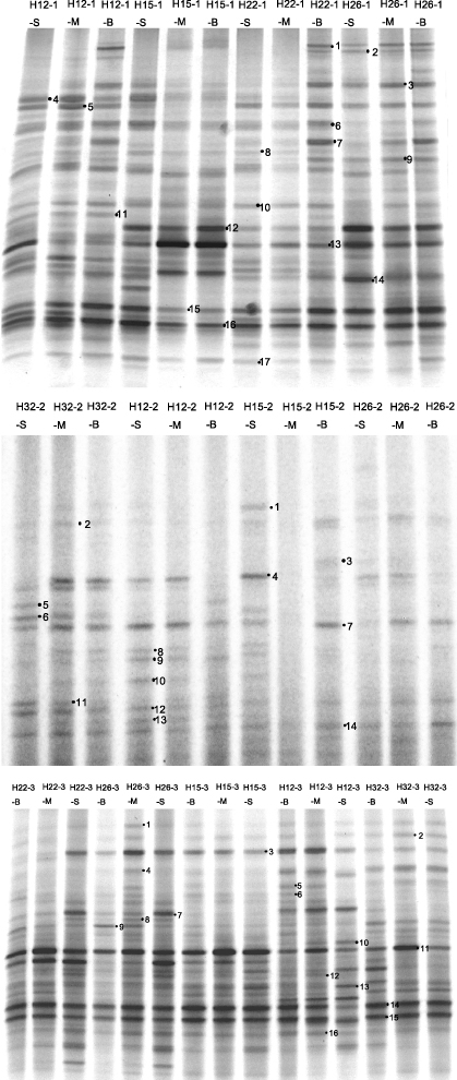
Figure 2. DGGE profiles showing bacterial communities of samples; each excised, cloned, and sequenced band is numbered. (-1, -2 and -3, samples collected in June, August and October, respectively; -S, -M, -B, samples collected from surface, middle and bottom layers, respectively.)
Download figure:
Standard image
Figure 3. Cluster analysis of the DGGE banding pattern performed with the NTSYS pc package using the unweighted pair group method, based on the presence or absence of each band. (-1, -2 and -3, samples collected in June, August and October, respectively; -S, -M, -B, samples collected from surface, middle and bottom layers, respectively.)
Download figure:
Standard imageForty-seven band sequences were affiliated to Gammaproteobacteria (twenty-eight band sequences), Cytophaga–Flavobacteria–Bacteroides (CFB) (twelve band sequences, mainly Flavobacteria subgroup), Deltaproteobacteria (two band sequences), Cyanobacteria (three band sequences) and Firmicutes (two band sequences) (table 2). Most of the sequences (89% of band sequences) were related to uncultured marine bacteria with high similarity (>96% similarity). The majority of sequences were from marine ecosystems, such as the inland sea of Japan, the NW Mediterranean Sea, the eastern subtropical North Pacific, the North Sea, Plum Island Sound Estuary, the Atlantic Ocean, the North Aegean Sea, the Guanabara Bay, Arctic sea ice, the Yellow Sea and Chesapeake Bay, except for three sequences from marine Alteromonas sp. KOPRI 11568 and one sequence from symbiotic associations in sea urchin, respectively.
Table 2. Sequence analysis of DGGE bands. (Note: CFB, Cytophaga–Flavobacteria–Bacteroides; -1, -2 and -3, samples collected in June, August and October, respectively.)
| Band no. | Accession no. | Phylogenetic affiliation | Closest relatives | Similarity (%) | Environmental description |
|---|---|---|---|---|---|
| 1-1 | EF467 883 | Gammaproteobacteria | Uncultured γ-proteobacterium DGGE band: HB02-12 (AB265 970) | 99 | Coastal seawater in the inland sea of Japan |
| 2-1 | EF433 338 | Deltaproteobacteria | Uncultured delta proteobacterium clone T42_65 (DQ436 705) | 99 | Seawater in the NW Mediterranean Sea |
| 3-1 | EF433 362 | Gammaproteobacteria | Alteromonas sp. KOPRI 11568 (AY138 988) | 100 | Marine Alteromonas sp. strain |
| 4-1 | EF433 358 | Gammaproteobacteria | Uncultured γ-proteobacterium DGGE band: SIS02-21 (AB265 980) | 99 | Coastal seawater in the inland sea of Japan |
| 5-1 | EF433 344 | Gammaproteobacteria | Uncultured γ-proteobacterium clone JL-ESNP-I14 (AY664 201) | 98 | Seawater in the eastern subtropical North Pacific |
| 6-1 | EF433 337 | CFB | Uncultured Flavobacteria bacterium clone NorSea82 (AM279 180) | 98 | Surface water in the North Sea |
| 7-1 | EF433 345 | Gammaproteobacteria | Alteromonas sp. KOPRI 11568 (AY138 988) | 98 | Marine Alteromonas sp. strain |
| 8-1 | EF433 355 | CFB | Uncultured Bacteroidetes bacterium clone NUD-28-1-2 (EU626 718) | 95 | Symbiotic associations in sea urchin |
| 9-1 | EF433 346 | Gammaproteobacteria | Uncultured γ-proteobacterium clone PI_4j5b (AY580 744) | 100 | Coastal seawater of Plum Island Sound Estuary |
| 10-1 | EF433 341 | Gammaproteobacteria | Uncultured γ-proteobacterium DGGE band: HB02-22 (AB265 981) | 97 | Coastal seawater in the inland sea of Japan |
| 11-1 | EF467 884 | Cyanobacteria | Uncultured cyanobacterium clone PI_4f9b (AY580 404) | 99 | Coastal seawater of Plum Island Sound Estuary |
| 12-1 | EF433 341 | Gammaproteobacteria | Uncultured γ-proteobacterium DGGE band: HB02-22 (AB265 981) | 97 | Coastal seawater in the inland sea of Japan |
| 13-1 | EF433 351 | Gammaproteobacteria | Uncultured γ-proteobacterium clone B649 (AM408 934) | 99 | Deep seawater in the Atlantic Ocean |
| 14-1 | EF433 350 | Firmicutes | Uncultured firmicute clone AEGEAN_247 (AF406 548) | 99 | Deep seawater in the North Aegean Sea |
| 15-1 | EF433 352 | CFB | Uncultured Flavobacteria bacterium clone MS024-1F (EF202 335) | 100 | Seawater in Boothbay Harbor, 1 m depth |
| 16-1 | EF433 342 | Gammaproteobacteria | Uncultured γ-proteobacterium clone T31_200 (DQ436 663) | 100 | Seawater in the NW Mediterranean Sea |
| 17-1 | EF433 335 | CFB | Uncultured Flavobacteria bacterium clone MS024-1F (EF202 335) | 98 | Seawater in Boothbay Harbor, 1 m depth |
| 1-2 | EF433 343 | Gammaproteobacteria | Uncultured γ-proteobacterium clone b1pl2F05 (EF092 639) | 100 | Subsurface seawater in Guanabara Bay |
| 2-2 | EF433 339 | Gammaproteobacteria | Uncultured γ-proteobacterium clone HF130_32J04 (EU361 591) | 99 | Ocean water in the Hawaii Ocean Time-series Station ALOHA |
| 3-2 | EF433 334 | Deltaproteobacteria | Uncultured delta proteobacterium clone T42_65 (DQ436 705) | 100 | Seawater in the NW Mediterranean Sea |
| 4-2 | EF467 882 | CFB | Uncultured Bacteroidetes bacterium clone T41_15 (DQ436 745) | 96 | Seawater in the NW Mediterranean Sea |
| 5-2 | EF433 345 | Gammaproteobacteria | Alteromonas sp. KOPRI 11568 (AY138 988) | 98 | Marine Alteromonas sp. strain |
| 6-2 | EF433 336 | Gammaproteobacteria | UnculturedVibrio sp. clone VDP57 (AY702 246) | 97 | Seawater in the Yellow Sea |
| 7-2 | EF433 354 | CFB | Uncultured Flavobacteria bacterium clone NorSea72 (AM279 212) | 98 | Surface water in the North Sea |
| 8-2 | EF433 341 | Gammaproteobacteria | Uncultured γ-proteobacterium DGGE band: HB02-22 (AB265 981) | 97 | Coastal seawater in the inland sea of Japan |
| 9-2 | EF433 340 | Gammaproteobacteria | Uncultured γ-proteobacterium DGGE band: SIS02-21 (AB265 980) | 99 | Coastal seawater in the inland sea of Japan |
| 10-2 | EF433 348 | Gammaproteobacteria | Uncultured γ-proteobacterium clone T32_198 (DQ436 678) | 98 | Seawater in the NW Mediterranean Sea |
| 11-2 | EF467 884 | Cyanobacteria | Uncultured cyanobacterium clone PI_4f9b (AY580 404) | 99 | Coastal seawater of Plum Island Sound Estuary |
| 12-2 | EF433 349 | Gammaproteobacteria | Uncultured γ-proteobacterium clone 5kpl2B07 (EF092 492) | 98 | Subsurface seawater in Guanabara Bay |
| 13-2 | EF433 342 | Gammaproteobacteria | Uncultured γ-proteobacterium clone T31_200 (DQ436 663) | 100 | Seawater in the NW Mediterranean Sea |
| 14-2 | EF433 353 | CFB | Uncultured Cytophaga sp. clone b1pl1D12 (EF092 710) | 95 | Subsurface seawater in Guanabara Bay |
| 1-3 | EF467 883 | Gammaproteobacteria | Uncultured γ-proteobacterium DGGE band: HB02-12 (AB265 970) | 99 | Coastal seawater in the inland sea of Japan |
| 2-3 | EF433 356 | Gammaproteobacteria | Uncultured γ-proteobacterium DGGE band: SIS02-21 (AB265 980) | 100 | Coastal seawater in the inland sea of Japan |
| 3-3 | EF433 369 | CFB | Uncultured Bacteroidetes bacterium clone 41 (AM748 216). | 96 | Seawater in the NW Mediterranean Sea |
| 4-3 | EF433 344 | Gammaproteobacteria | Uncultured γ-proteobacterium clone JL-ESNP-I14 (AY664 201) | 98 | Seawater in the eastern subtropical North Pacific |
| 5-3 | EF433 360 | Gammaproteobacteria | Uncultured γ-proteobacterium clone PI_RT72 (AY580 804) | 99 | Coastal seawater of Plum Island Sound Estuary |
| 6-3 | EF433 359 | Gammaproteobacteria | Uncultured γ-proteobacterium clone 5kpl1H10 (EF092 475) | 100 | Subsurface seawater in Guanabara Bay |
| 7-3 | EF433 336 | Gammaproteobacteria | Uncultured Vibrio sp. clone VDP57 (AY702 246) | 97 | Seawater in the Yellow Sea |
| 8-3 | EF433 370 | Gammaproteobacteria | Pseudoalteromonas sp. Bsi20671 (EF198 395) | 100 | Arctic sea ice |
| 9-3 | EF433 357 | Gammaproteobacteria | Uncultured γ-proteobacterium clone T32_61 (DQ436 669) | 97 | Seawater in the NW Mediterranean Sea |
| 10-3 | EF467 884 | Cyanobacteria | Uncultured cyanobacterium clone PI_4f9b (AY580 404) | 99 | Coastal seawater of Plum Island Sound Estuary |
| 11-3 | EF433 361 | CFB | Uncultured Bacteroidetes bacterium clone T42_183 (DQ436 774) | 100 | Seawater in the NW Mediterranean Sea |
| 12-3 | EF433 351 | Gammaproteobacteria | Uncultured γ-proteobacterium clone B649 (AM408 934) | 99 | Deep seawater in the Atlantic Ocean |
| 13-3 | EF433 350 | Firmicutes | Uncultured firmicute clone AEGEAN_247 (AF406 548) | 99 | Deep seawater in the North Aegean Sea |
| 14-3 | EF433 352 | CFB | Uncultured Flavobacteria bacterium clone MS024-1F (EF202 335) | 100 | Seawater in Boothbay Harbor, 1 m depth |
| 15-3 | EF433 371 | CFB | Uncultured Bacteroidetes bacterium clone CB01F12 (EF471714) | 95 | Seawater in Chesapeake Bay |
| 16-3 | EF433 335 | CFB | Uncultured Flavobacteria bacterium clone MS024-1F (EF202 335) | 98 | Seawater in Boothbay Harbor, 1 m depth |
Comparison of bacterial community structure among the samples revealed by DGGE is displayed in figure 4 (as percentages of the different groups based on the density of their correlated DGGE bands). Two bacterial clusters, Gammaproteobacteria and CFB, were the dominant groups in all samples in June, August and October. However, the two dominant clusters presented different proportions among the three months. The average percentage of Gammaproteobacteria decreased from 63% in June to 49% in August and to 22% in October whereas the average percentage of CFB increased from 29% in June to 48% in August and to 63% in October. A higher percentage of Deltaproteobacteria was observed in samples in October (8% on average) than other samples in June and August (both 1% on average). The Firmicutes cluster was observed in samples in June and October (both 6% on average) but not in August. Small numbers of Cyanobacteria band sequences were found in the three months, on average 1%, 2% and 1%, respectively. Notably, the percentages of Cyanobacteria sequences were relatively higher at stations H32 (5% on average) and H12 (3% on average) in August, up to 12% in H32-2-S (figure 4).

Figure 4. Bacterial community structures of samples based on the quantitative analysis of the DGGE bands. (-1, -2 and -3, samples collected in June, August and October, respectively; -S, -M, -B, samples collected from surface, middle and bottom layers, respectively.)
Download figure:
Standard image3.3. Relation between bacterial community composition and environmental variables
The eigenvalues of the ordination analyses are shown in table 3. The sum of all eigenvalues indicated an overall variance in the dataset of 0.743, 2.509 and 0.85 in June, August and October, respectively. The sum of all canonical eigenvalues indicated the total variation explained by environmental variation, accounting for 0.621, 1.944 and 0.525 in June, August and October, respectively. Species–environment correlations in samples in three months were high (especially for axes 1, >90%), indicating a strong relationship between species and environmental variables (table 3). Concerning the variance of species data, the first axis explained 33.6%, 28.0% and 21.9% of the total variation, and all four axes explained 69.1%, 66.8% and 53.6% in June, August and October, respectively. The variation of the species–environment relation explained by the first axis was 40.3%, 36.1% and 35.4% in June, August and October, respectively.
Table 3. Eigenvalues and variance decomposition for CCA in samples of June, August and October, respectively.
| Samples | Axes | Eigenvalues | Species–environment correlations | Cumulative percentage variance of species data | Cumulative percentage variance of species–environment relation |
|---|---|---|---|---|---|
| June | Axis 1 | 0.250 | 0.997 | 33.6 | 40.3 |
| Axis 2 | 0.130 | 0.899 | 51.2 | 61.2 | |
| Axis 3 | 0.089 | 0.96 | 63.1 | 75.6 | |
| Axis 4 | 0.044 | 0.999 | 69.1 | 82.7 | |
| August | Axis 1 | 0.701 | 0.973 | 28.0 | 36.1 |
| Axis 2 | 0.479 | 0.963 | 47.0 | 60.7 | |
| Axis 3 | 0.264 | 0.844 | 57.6 | 74.3 | |
| Axis 4 | 0.232 | 0.964 | 66.8 | 86.2 | |
| October | Axis 1 | 0.186 | 0.98 | 21.9 | 35.4 |
| Axis 2 | 0.131 | 0.935 | 37.3 | 60.3 | |
| Axis 3 | 0.084 | 0.912 | 47.1 | 76.3 | |
| Axis 4 | 0.055 | 0.854 | 53.6 | 86.8 |
Biplot scalings of CCA with inter-sample distances are shown in figure 5. In June, axis 1 represented a strong gradient caused by DOC (figure 5(a)), indicated by the correlation coefficient of −0.7952. Axis 2 represented a gradient due to the environmental factor nitrite (figure 5(a)), as indicated by its correlation coefficient of −0.5122. Based on the 5% level in a partial Monte Carlo permutation test, DOC (P = 0.0080, F = 3.16) and temperature (P = 0.0240, F = 2.42) were the significant environmental variables, and the two factors alone provided 29.0% and 19.3% of the total CCA explanatory power, respectively. In August, axis 1 and axis 2 represented a gradient caused by nitrite and phosphate (figure 5(b)), indicated by the correlation coefficient of 0.8952 and −0.4834, respectively. Nitrite was the significant environmental variable (P = 0.0140, F = 2.93), which provided 32.0% of the total CCA explanatory power. In October, the variables salinity and pH contributed particularly to the gradient of axis 1 and axis 2 (figure 5(c)), as indicated by the correlation coefficients of −0.8682 and −0.7127, respectively. However, none of the variables displayed significant influence on the bacterial community at the 5% level.
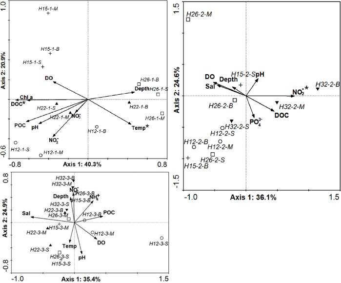
Figure 5. Canonical correspondence analysis (CCA) ordination diagram of bacterial communities associated with environmental variables. Environmental variables were indicated as arrows. DGGE samples were indicated as (○) samples at station H12, ( + ) samples at station H15, (▴) samples at station H22, (□) samples at station H26, and (▾) samples at station H32. Environmental variables marked with asterisks were significant (P < 0.05). (Temp, temperature; Sal, salinity; DO, dissolved oxygen; DOC, dissolved organic carbon; POC, particulate organic carbon; -1, -2 and -3, samples collected in June, August and October, respectively; -S, -M, -B, samples collected from surface, middle and bottom layer, respectively.)
Download figure:
Standard image4. Discussion
Bacterial community composition in the hypoxia area has been reported (Stevens and Ulloa 2008). However, little is known about the effects of environmental factors on the diversity and distribution of bacteria. CCA is powerful in detecting the relationship between microbiological community composition and environmental factors (Salles et al 2004, Haukka et al 2006, Sapp et al 2007). Several environmental parameters, such as total phosphorus, organic matter and pH, have been considered as the key factors driving the changes in community composition in aquatic ecosystems (Lindström and Bergström 2005, Haukka et al 2006). CCA analysis indicated that salinity, not dissolved oxygen, had a significant effect on the archeal community composition in the Changjiang Estuary hypoxia area and the adjacent ECS (Liu et al 2011). Whether dissolved oxygen significantly influenced bacterial community composition in this area has received little attention. In this study, the CCA results indicated no significant relationship between dissolved oxygen and the bacterial community structure.
In this study, the environmental factors significantly influencing bacterial community structure are different in the three months. In June, DOC was one of the significant environmental effectors. Samples from surface and middle layers at offshore stations H12-1 and H22-1 with higher DOC concentrations grouped together through clustering analysis (table 1 and figure 3), which also suggested that DOC greatly influenced bacterial community. These results might be explained because phytoplankton grew in bloom and could produce massive DOC in offshore area with rich nutrients. Temperature was another significant environmental factor, which might be explained by the influences of the Yellow Sea cold water mass on bacterial community composition. Zhang et al (2011) reported that bacterial community structure was significantly influenced by cyclonic eddy perturbations, which introduce hydrographic and chemical changes inside of eddies. In August, nitrite significantly influenced bacterial community composition and dissolved oxygen had no significant effect on it (P = 0.2300). Hypoxia is especially associated with denitrification (Codispoti et al 2001), and an increase in nitrate concentration can dramatically promote denitrification (Middelburg and Levin 2009). Higher nitrite concentration was observed in samples H12-2-M/H12-2-B and H32-2-M/H32-2-B. Based on these results, it was suggested that hypoxia had no direct significant effect on bacterial community but an indirect influence in this study. In October, no environmental variables measured were significant effective factors on the bacterial community, which might be determined by other biotic and abiotic factors. Besides physical and chemical variables, phytoplankton composition, grazing and viral infection play important roles in shaping bacterial community structure (Beardsley et al 2003, Pinhassi et al 2004, Grossart et al 2005, Bouvier and del Giorgio 2007, Weinbauer et al 2007). The environmental heterogeneity in season in the Changjiang Estuary and its adjacent area in the ECS, such as seasonal hydrodynamic conditions and riverine input of nutrients (Chen et al 1999), might be the reason for the difference in environmental factors significantly determining the bacterial community in the three months.
The bacterial community was predominantly characterized by bacteria affiliated to Alphaproteobacteria (the marine SAR11 clade) and Gammaproteobacteria (to thiotrophic γ-symbionts) in the oxygen minimum zone of the eastern tropical South Pacific (Stevens and Ulloa 2008). In comparison, the bacterial community in the Changjiang Estuary hypoxia area was dominated by Gammaproteobacteria and CFB by DGGE band sequencing analysis. Differences in mechanisms for the occurrence of oxygen depletion and in oxygen concentrations between the two areas might be one of the reasons for the different bacterial community compositions (Daneri et al 2000, Helly and Levin 2004, Zhu et al 2011). Alphaproteobacterial sequence (such as SAR11 clade), which usually is dominant in surface seawaters (Morris et al 2002), was not found in this study. This might be due to the bias of DGGE band sequencing analysis. Although DGGE is a useful molecular technology in monitoring the dynamics of a microbial community and comparison of multiple samples (Sapp et al 2007, Zhang et al 2007, Zeng et al 2009), DGGE band sequencing provides limited phylogenetic diversity information and only predominant populations in the assemblage could be obtained (Muyzer et al 1993, Murray et al 1996, Feng et al 2009) also reported on the bacterial community in the Changjiang Estuary and the ECS, which was dominated by Gammaproteobacteria, Alphaproteobacteria and Deltaproteobacteria. Sampling site and sampling time were different between the two studies in Changjiang Estuary and the ECS, the former investigated in coastal and pelagic sites in June, August and October and the latter mainly in coastal sites in May and October. Different bacterial assemblages were harbored along particular estuarine, geochemical and eutrophication gradients from offshore to the pelagic area. In addition, two different molecular methods were applied, DGGE used in the former and a clone library in the latter.
In this study, CFB (mainly Flavobacteria subgroup) was the dominant cluster. Cytophaga–Flavobacteria are chemoorganotrophic, mainly aerobic, and are especially proficient in degrading polymeric organic matter (Kirchman 2002). From the previous results (Wei et al 2007, Zhu et al 2011), organic matter decomposition contributes greatly to oxygen depletion in the Changjiang Estuary area. The high abundance of CFB (mainly Flavobacteria subgroup) in this study suggested that this bacterial assemblage played an important role in biochemical degradation processes in the Changjiang Estuary hypoxia area. A relationship between some bacterial clusters (such as CFB) and oxygen depletion was implied. Abundance of CFB increased twofold from June to October, which contributed greatly to seasonal changes of the bacterial community. This variation of CFB abundance might be related to availability of polymeric organic matter from seasonal terrestrial input or alga-derived metabolites and detritus. As we all know, cyanobacteria are photosynthetic and oxygen-producing organisms (Ting et al 2002). In this study, Cyanobacteria in samples at hypoxia stations in August possessed higher abundances than other samples (especially up to 12% in H32-2-S), which suggested that Cyanobacteria contributed to photosynthesis in the hypoxia area.
Acknowledgments
We are grateful to Dr Yuhe Tong for constructive comments. This study was supported by the Major State Basic Research Development Program of China (No. 2011CB409804), the Natural Science Foundation of China (No. 41121064) and the National Non-profit Institute Research Grant of CATAS-ITBB from the Chinese Government (No. ITBB11-0208).