

Abstract
Severe convective storms cause catastrophic losses each year in the United States, suggesting that any predictive capability is of great societal benefit. While it is known that El Niño and the Southern Oscillation (ENSO) influence high impact weather events, such as a tornado activity and severe storms, in the US during early spring, this study highlights that the influence of ENSO on US severe storm characteristics is weak during May–July. Instead, warm water in the Gulf of Mexico is a potential predictor for moist instability, which is an important factor in influencing the storm characteristics in the US during May–July.
Export citation and abstract BibTeX RIS

Original content from this work may be used under the terms of the Creative Commons Attribution 3.0 licence. Any further distribution of this work must maintain attribution to the author(s) and the title of the work, journal citation and DOI.
1. Introduction
Severe convective storms cause catastrophic losses each year in the United States; yet, predicting extreme weather remains a daunting challenging. Within a season or a month, individual extreme weather events are not predictable. However, the large-scale atmospheric conditions upon which extreme weather is superimposed may be more (or less) likely to be predictable on longer time scales. Indeed, large-scale atmospheric conditions have been used to establish relationships between severe weather occurrence and the associated favorable environments (e.g., Gray 1979, Brooks et al 1994, 2003b, Craven and Brooks 2004, Shepherd et al 2009, Tippett et al 2012, 2014, Allen et al 2015). Here we use the NCAR Community Climate System Model version 4.0 (CCSM4) forecasts and North American Regional Reanalysis (NARR) for the period of 1982–2011, and examine whether we can predict the seasonal changes in the likelihood of moist instability, which is an important ingredient in influencing the storm characteristics in the US. Since May is the peak month for tornado activity in the US (e.g., Brooks et al 2003a, Tippett et al 2012, see also supplementary material figure S1), this study focuses on May–July (MJJ). The goal here is to assess whether we can accurately forecast the May–July large-scale environment (e.g., moist instability) that is favorable for high impact weather such as tornado activity in the US.
Although multiple factors were analyzed to determine the favorability of environmental conditions for severe weather occurrence previously (e.g., Gensini and Ashley 2011, Tippett et al 2012), we use convective available potential energy (CAPE) as the background state in which changes produce conditions that are more (or less) favorable for severe weather. This approach is, in part, motivated by the colocation of CAPE and the geographical distribution of tornadoes in the US during MJJ (figure 1). There are also direct physical relationships that motivate the use of variations in CAPE as predictor of increased or decreased probability of severe weather. CAPE is a measure of the vertically integrated buoyant energy available for storm formation, and indeed, severe storms occur most readily when CAPE and vertical wind shear are both large in a local environment (Rasmussen and Blanchard 1998, Craven and Brooks 2004, Brooks and Dotzek 2008, see also supplementary material figures S2 and S3). In terms of the annual cycle, large values of CAPE first emerge along the Gulf Coast in March (supplementary material figure S3). The areas of climatologically high CAPE then extend north and northeastward through August. The evolution of CAPE is very similar to observed convective precipitation (not shown); and further it agrees with the geographical distribution of tornadoes (figure 1, see also supplementary material figures S1 and S3). On the other hand, the area of relatively strong shear, which is the other ingredient of severe storms, migrates northward during warm months, resulting in weak shear (both in mean and variance) in the US during MJJ (supplementary material figure S4). As a result, CAPE alone displays a similar distribution and evolution as the combination of CAPE and shear in the US during MJJ (figures 1 and supplementary material S1–S3), indicating that CAPE is a reasonable predictor for the increased or decreased probability of severe storms (or tornado activity) in the US during MJJ. It should be emphasized that we are not suggesting predictability for specific severe weather events. We are, however, proposing the possibility of probabilistically predicting changes in the background state that makes severe weather more (or less) probable.
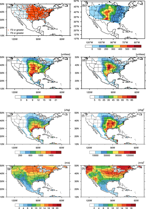
Figure 1. May–July (MJJ) climatology and variance, May 1982–April 2011. (a) Distribution of MJJ tornadoes (b) total number of tornadoes in each state. (c) Climatology and (d) variance of combination of convective available potential energy (CAPE) and shear, (e) climatology and (f) variance of CAPE, (g) climatology and (h) variance of shear from North American Regional Reanalysis (NARR). Southeast US region in this study is shown as a box in figure 1(f).
Download figure:
Standard image High-resolution imageIn figure 2, CAPE varies widely from year to year. For example, CAPE in 2011 is anomalously large, suggesting a higher chance of severe storms such as tornado activity. Indeed, 2011 was an exceptionally destructive year for tornadoes in the US. In contrast, CAPE in 1988 was less than climatology, suggesting 1988 would have a reduced probability for tornadoes as was observed. Motivated by the fact that CAPE appears to be related to severe storms as moisture instability is an important ingredient in influencing storm characteristics, we ask: can we predict seasonal variability of CAPE in the US during May–July? We choose to use actual climate forecasts (see data and method section) so that one-to-one comparisons with observational estimates are possible.
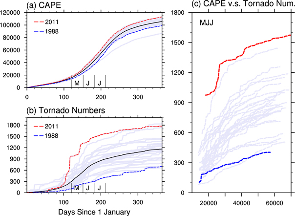
Figure 2. Accumulated CAPE and accumulated number of tornadoes in the US for 1982–2011. The lavender shading represents (a) CAPE and (b) tornado numbers for each year, and the climatology is shown as a bold solid black line. Accumulated MJJ CAPE versus accumulated MJJ tornado numbers are shown in figure 2(c). MJJ indicates May June and July. Individual years 2011 (red) and 1988 (blue) are shown as dashed lines. CAPE is obtained from NARR. Tornado data are obtained from Severe Weather Database (SWD) from NOAA. Numbers are counted for tornadoes F0 or greater on Fujita–Person scale.
Download figure:
Standard image High-resolution image2. Data and method
2.1. Model and observations
The model used for this study is the NCAR Community Climate System Model version 4.0 (CCSM4.0). The performance of the model based on a complete set of metrics is described in a J. Climate special collection (e.g., Gent et al 2011), and is currently being used for routine real-time predictions (http://cpc.ncep.noaa.gov/products/NMME/) as part of North American Multi-Model Ensemble (NMME) (Kirtman et al 2014). In this study, the ten ensemble members of CCSM4 are initialized every May 1st and forecasted until the following April 30th over the period 1982–2011.
For the observational estimates, North American Regional Reanalysis (NARR, Mesinger et al 2006) dataset are used unless otherwise specified. NARR data are provided on a 32 km Lambert conformal grid, which we interpolate to the resolution of CCSM4 (1° × 1° latitude–longitude grid). The data are obtained from the Earth System Research Laboratory Physical Sciences Division (http://esrl.noaa.gov/psd/data/gridded/data.narr.html) through an anonymous ftp. For the regions outside the North America, the Advanced Very High Resolution Radiometer (AVHRR) global Blended sea surface temperature (SST) (level 4, Reynolds et al 2007) is used. The daily SST data are on 0.25° longitude × 0.25° latitude global grid and cover the period 1982-present. The SST data are obtained from NOAA National Climatic Data Center through ftp (ftp://ftp.nodc.noaa.gov/pub/data.nodc/ghrsst/L4/GLOB/NCDC/AVHRR_OI).
2.2. CAPE, GoM and Niño 3.4 indices
The CAPE indices are defined as area-averaged CAPE anomalies over the region of interest—in this case all of the US and separately the Southeast US (30–40°N, 85–100°W, figure 1(f)). The GoM index is an area-averaged SST anomaly in the Gulf of Mexico (20–30°N, 82°W–98°W). The Niño 3.4 index is calculated by averaging SST anomalies over the region between 120°W–170°W and 5°S–5°N. SST is detrended and ocean (land)-only grids are used to calculate GoM (CAPE) index. CCSM4 CAPE is calculated at the same 26 vertical levels as NARR using a freely available the NCL function. NARR CAPE is downloaded from its website at http://esrl.noaa.gov/psd/.
3. Results and discussion
Since relatively high CAPE emerges in the Gulf of Mexico and Gulf Coast in early spring, and then expands north and northeastward during the primary tornado outbreak period, we correlated CAPE anomalies in the US to SST anomalies in the Gulf of Mexico. The linear relationship between them is examined by introducing CAPE and GoM indices, which are area-averaged CAPE anomalies in the US and SST anomalies in the Gulf of Mexico, respectively (see method section for details).
Scatter diagrams of the CAPE indices with GoM and Niño 3.4 indices are shown in figure 3. In figures 3(a) and (b), as SST in the Gulf of Mexico becomes anomalously warmer, CAPE in the US tends to become higher in both the forecasts (left) and the observational estimates (right). Correlations are slightly higher in the CCSM4 predictions than in the observational estimates; and correlations are higher in the Southeast US, where the strongest CAPE variation is found compared with correlations calculated from all of the US. The same analysis is performed with seasonal mean CAPE data as opposed to the accumulated CAPE shown in figure 3 (supplementary material figure S5), and also with the combination of CAPE and shear (not shown); and the results are robust. Figure 3 further shows that US CAPE during MJJ does not have contemporaneous relationships with SST in the Niño 3.4 region (figures 3(c) and (d)). Further, SST in the Niño 3.4 region does not have contemporaneous as well as lagged relationships with MJJ US CAPE (supplementary material table S1). SST in the Niño 3.4 region does not have a contemporaneous relationship with SST in the Gulf of Mexico during MJJ either (not shown).
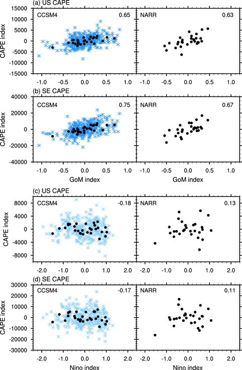
Figure 3. Scatter diagrams of the CAPE indices with the GoM and Niño 3.4 indices during MJJ from forecasts (CCSM4) and observational estimates (NARR). The CAPE indices are calculated by averaging daily CAPE anomalies in the US (US CAPE) and in the southeast US (SE CAPE). The GoM index and Niño 3.4 index are each an area-averaged SST anomaly in their representative regions. Individual forecast ensemble members are shown as blue asterisks and the ensemble mean is shown as black dots. The correlations between two indices are shown in the upper right corner in each box.
Download figure:
Standard image High-resolution imageThe apparent lack of a contemporaneous relationship between Niño 3.4 SST and US CAPE requires further discussion, in particular when El Niño and the Southern Oscillation (ENSO) phase is recognized to play roles in tornado activities in the US (e.g., Cook and Schaefer 2008, Lee et al 2013, Allen et al 2015). In the study of Cook and Schaefer (2008), intense tornado activity was found in a southwest–northeast band from Louisiana to Michigan during La Niña winters. In contrast, tornado activity was restricted to areas immediately adjacent to the Gulf of Mexico during El Niño winters. However, the overall tornado activity was most intense during ENSO neutral years, suggesting that US tornado activity is weakly correlated with ENSO. Lee et al (2013) also showed a weak correlation between US tornado activity and Niño 3.4 index. Additionally, Lee et al (2013) identified an optimal ENSO pattern that relates to the top ten extreme tornado years in the US during April–May, 1950–2010. However, the number of intense tornadoes did not decrease during the negative phase of optimal ENSO pattern years. We note that, consistent with our results, the SST in the Gulf of Mexico in their study was warmer than normal during the active tornado years (e.g., figure 7 from Lee et al 2013). More recently, Allen et al (2015) showed the ENSO influence on hail and tornado frequencies in the US during March–May. The relationship between ENSO and US spring tornado activity in their study was because the winter ENSO conditions often persisted into early spring. The CAPE index in our study was calculated for all of US and separately for the Southeast US, and did not show any correlations with ENSO during MJJ (figures 3(c) and (d)). However, we do not exclude the possibility that there are correlations between CAPE and ENSO for other regions of US during MJJ.
It is also possible that there are correlations between MJJ US CAPE and the antecedent winter (DJF) ENSO as shown in Allen et al (2015). However, MJJ is found to be the months in which ENSO has the least influence on SST in the Gulf of Mexico and thus CAPE in the US in figure 4. In contrast, the influence of antecedent winter ENSO on the Gulf of Mexico SST is the strongest during February–April (figure 4 red line), and it becomes weaker if strong ENSO years were excluded from the analysis (figure 4 red versus orange lines). The antecedent winter ENSO possibly could affect one or both ingredients of tornadoes (CAPE and shear) in the US during those months through SST and shear variability, which are associated with the southward shift of jet streams (Weaver et al 2012). The more frequently observed stronger tornadoes (i.e., larger E/F scale) during February–April/May (supplementary material figure S1) could be related to ENSO.
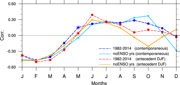
Figure 4. Contemporaneous and antecedent ENSO influence on the Gulf of Mexico SST. Correlations between SST anomalies in the Gulf of Mexico and Niño 3.4 regions are calculated first from all years 1982–2014 and second by excluding strong ENSO years. Strong ENSO years used are 1982/1983, 1988/1989, 1997/1998, 2011/2012. Three months mean values are used to calculate the correlation, for example, correlation shown in May (M) is calculated from SST anomalies during May–July months.
Download figure:
Standard image High-resolution imageMotivated by the results in figure 3, which showed a linear relationship between SST anomaly in the Gulf of Mexico and CAPE in the US, we diagnosed the spatial patterns associated with this correlation (supplementary material figure S6). To obtain the characteristic patterns of CAPE associated with anomalously warmer SST in the Gulf of Mexico, MJJ CAPE anomalies were averaged for all years of positive GoM indices. When the Gulf of Mexico SST is anomalously warm, positive CAPE anomalies are found in the US (see supplementary material figure S6). Similarly, cold Gulf of Mexico SST is associated with reduced CAPE over the US (not shown). The maximum positive CAPE anomalies are detected along the Gulf Coast, Tornado Alley and Florida, where relatively high CAPE variance and high frequency of tornadoes are found, implying that CAPE anomalies in the US are contemporaneously related to the SST anomalies in the Gulf of Mexico during MJJ. The forecasts show similar patterns to the observational estimates, but notably do not extend as far north into the US. We further examined correlations between GoM index and US CAPE during MJJ and partial correlations between GoM index and US CAPE while the influence of Niño 3.4 SST held fixed. The resulted correlation maps were almost identical to supplementary material figure S6 (not shown), confirming the little influence of ENSO on US tornado activity during MJJ.
The possible mechanisms for the high correlations between GoM SST and US CAPE anomalies were examined via the composite maps of low-level moisture, meridional-winds, and northward moisture transport anomalies (supplementary material figure S7). The positive GoM index years are characterized by increased low-level moisture and southerlies as well as increased low-level northward moisture transports to the east of Rocky Mountains (supplementary material figures S7(a)–(f)). On the other hand, the negative GoM index years are associated with decreased low-level moisture, northerlies, and reduced GoM to US moisture transports (supplementary material figures S7(g)–(l)). Supplementary material figure S7 essentially suggests that moisture transports from GoM to US under the warmer GoM SST conditions are associated with an increase in US CAPE during MJJ. The results agree with previous studies in that the GoM is viewed as a source of moisture for US (Hastenrath 1966, Rasmusson 1967, Mo et al 1995, Bosilovich and Schubert 2002, Mestas-Nuñez et al 2007, Muñoz and Enfield 2011, Lee et al 2013, Dirmeyer et al 2014) and that the Intra-Americas low-level jets play a role on the high impact weather in the US (e.g., Mo et al 1995, Hu and Feng 2001, Mestas-Nuñez et al 2005, 2007, Muñoz and Enfield 2011, Lee et al 2013, Nayak et al 2016).
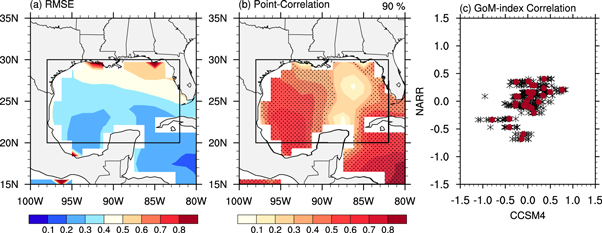
Given the importance of SST in the Gulf of Mexico, how well the SST anomaly in the Gulf can be predicted? The seasonal prediction skill is assessed by point-correlation and root-mean-squared-error (RMSE) between predicted and observed SST anomalies in the Gulf of Mexico (figure 5). The RMSE between the observed and predicted SST anomalies in the Gulf of Mexico is relatively small (smaller than 0.5 °C) in most of the Gulf, and increases to the north (figure 5(a)). Point correlations are relatively high (higher than 0.3, statistically significant at the 90% confidence level) except for regions from Yucatan Peninsula to Tallahassee, Florida (figure 5(b)). The overall correlation between forecasts and observational estimates is about 0.42. The correlation between the observed and the predicted GoM-index is 0.51 (figure 5(c)).
Figure 5. Seasonal prediction skill of SST in the Gulf of Mexico. (a) Root-mean-squared error (RMSE) and (b) point-correlation between observed and predicted SST anomalies for 1982–2011. The stippled areas in figure 5(b) are statistically significant at the 90% confidence level. (c) Scatter diagram of observed and predicted area-averaged SST anomalies in the Gulf of Mexico (GoM index). The area used for calculating the GoM index is shown as a box in figures 5(a) and (b). Individual forecast ensemble members are shown as black asterisks and the ensemble mean is shown as red dots. The correlations between two indices are shown in the upper right corner.
Download figure:
Standard image High-resolution image
4. Summary and conclusions
Severe storms threaten lives throughout the United States (US) every year, suggesting that any predictive capability is of large societal benefit. While it is well recognized that predicting individual tornado outbreaks or severe storms is only possible a few hours in advance, the large-scale background atmospheric conditions that influence the likelihood of severe storms maybe more predictable. In this study, CAPE is used as background state in which variations create conditions that are more or less favorable for severe weather occurrence, noting that moist instability is an important ingredients in influencing the storm characteristics. We are not suggesting that specific storms can be predicted with this approach.
Here we analyzed 30 years of May–July (MJJ) predicted CAPE from May 1st initialized forecasts from NCAR Community Climate System Model version 4.0 (CCSM4). The forecasts were compared with observational estimates from NARR. The results show that an area-averaged SST anomaly in the Gulf of Mexico (GoM index) is a possible predictor for forecasting CAPE anomalies in the US: the warmer the SST in the Gulf of Mexico, the higher CAPE in the contiguous US during MJJ seasons. The mechanism behind the correlation between GoM index and CAPE in the US is due to the variations in moisture transport from the Gulf of Mexico to US. Considering our current ability to predict SST in the Gulf of Mexico compared with the difficulty of predicting high impact weather in the US, the findings are promising for the seasonal prediction of enhanced or decreased severe storms (e.g., tornado activity) in the US during May–July using the Gulf of Mexico SST. This study further emphasizes that the influence of ENSO (contemporaneous as well as antecedent winter ENSO) on the Gulf of Mexico SST (and ultimately high impact weather in the US) is weak during MJJ, and thus, there is no clear relationship between US CAPE and ENSO during MJJ.
Acknowledgments
This research was supported by NOAA grants NA14OAR4830127, NA12OAR4310089 and NA10OAR4320143. EJ would like to thanks all individuals and groups who contribute to collect, produce and maintain the observational estimates and model data that used in this study. We thank three anonymous reviewers for their constructive comments on the manuscript.