


Abstract
Corporations and other multinational institutions are increasingly looking to evaluate their innovation and procurement decisions over a range of environmental criteria, including impacts on ecosystem services according to the spatial configuration of activities on the landscape. We have developed a spatially explicit approach and modeled a hypothetical corporate supply chain decision representing contrasting patterns of land-use change in four regions of the globe. This illustrates the effect of introducing spatial considerations in the analysis of ecosystem services, specifically sediment retention. We explored a wide variety of contexts (Iowa, USA; Mato Grosso, Brazil; and Jiangxi and Heilongjiang in China) and these show that per-area representation of impacts based on the physical characterization of a region can be misleading. We found two- to five-fold differences in sediment export for the same amount of habitat conversion within regions characterized by similar physical traits. These differences were mainly determined by the distance between land use changes and streams. The influence of landscape configuration is so dramatic that it can override wide variation in erosion potential driven by physical factors like soil type, slope, and climate. To minimize damage to spatially-dependent ecosystem services like water purification, sustainable sourcing strategies should not assume a direct correlation between impact and area but rather allow for possible nonlinearity in impacts, especially in regions with little remaining habitat and highly variable hydrological connectivity.
Export citation and abstract BibTeX RIS

Original content from this work may be used under the terms of the Creative Commons Attribution 3.0 licence. Any further distribution of this work must maintain attribution to the author(s) and the title of the work, journal citation and DOI.
1. Introduction
With a world population estimated to reach nine billion people by 2050, and changing consumption patterns towards more animal protein-rich diets, food demand is projected to double by 2050 (Tilman et al 2011). Meeting this demand while limiting adverse environmental impacts is a global challenge, but a combination of agricultural intensification and expansion responses are anticipated. Corporate commitments to sustainability provide an increasingly powerful means of addressing the impacts of these responses to increasing demand on natural systems (Chaplin-Kramer et al 2015a, Jones et al 2015, Kareiva et al 2015). Companies make decisions that influence the location of agricultural production worldwide, through their choice of ingredients (product innovation) and suppliers (procurement decisions). Therefore, they directly or indirectly affect where land-use change and its impacts take place.
The environmental impacts of product development and procurement decisions are typically evaluated using life cycle assessment (LCA) based methods, to help identify ingredient and technology choices associated with lowest impacts (Hellweg and Milà i Canals 2014, Sim et al 2016). For bio-based products, agriculture is often identified as a life cycle hotspot (Notarnicola et al 2012, Kulak et al 2013, Milà i Canals et al 2013) for a range of environmental impacts, recognizing agricultural management, land use and land use change as key drivers of impact. Current LCA approaches model land-use change or transformation and occupation on an area basis (de Baan et al 2012, Flynn et al 2012, Muñoz et al 2013) as a proxy for impacts on ecosystem services. However, the provisioning of a variety of ecosystem services depends not only on the total area of habitat, but also on the spatial arrangement of habitats within a landscape (Polasky et al 2008, Nelson et al 2010, Mitchell et al 2014, Chaplin-Kramer et al 2015b). Consequently, assuming uniformity when interpreting the land transformation into impacts on ecosystem services is an over-simplification and could result in erroneous decision-making.
Water purification is an ecosystem service that is especially sensitive to the spatial pattern of land-use change because areas near to a watercourse often play more of a role in retaining or exporting soils and nutrients than those further away (Brauman et al 2007, Gardner et al 2011). In particular, management practices such as riparian buffers are very effective at retaining sediment and nutrient from upslope agricultural areas (Liu et al 2008, Yuan et al 2009, Poeppl et al 2012). Although improved management practices can reduce the levels of run-off from land, the placement of agriculture versus natural habitat in relation to watercourses affects the degree to which sediments, nutrients and chemicals reach major waterways (Strauss et al 2007, Dosskey and Qiu 2011, Rabotyagov et al 2014). Agricultural expansion therefore poses a threat to water quality and it is not merely the total area of expansion, but also its arrangement on the ground, that will ultimately determine the impacts to aquatic ecosystems and critical water sources for people. Sediment and sediment-related discharges (including runoff) contribute the majority of nitrogen, phosphorus, and suspended solids to waterways, causing increased treatment and dredging costs that may approach or exceed the costs of soil loss to agricultural production (Holmes 1988). In some cases these costs have been found to increase at a disproportionate rate to the deforestation causing the erosion (1.58%–1% in India; Singh and Mishra 2014).
In this paper, we demonstrate the importance of spatially resolved impact assessment to sediment export. This analysis explores the degree to which different spatial patterns of land-use change really matter for sediment export, compared to broader physical differences between regions, like climate, soil and slope. Using scenarios of agricultural expansion in four regions, we demonstrate the importance of considering spatially explicit patterns of land-use change on sediment export. Soil loss is an impact category that is not addressed in standard LCA methods, but an approach has recently been developed to include this important driver of water quality in such sustainability assessments (Saad et al 2013). We invoke a simple but spatially-explicit model, which we suggest can be utilized in corporate and other global contexts to expand on and supplement current land-use change impact assessments in LCA. In addition to supply chain decisions, we expect this approach to be applicable to many other global decision-making contexts that are apt to use regional proxies when comparing potential impacts of change across regions and would benefit from more spatially-explicit methods, such as watershed screening approaches for conservation agencies (McDonald et al 2015) and global prioritization strategies for development banks (Mandle et al 2015).
2. Methods
To explore how landscape characteristics and patterns of agricultural expansion impact sediment export, we applied the InVEST sediment delivery model (Sharp et al 2015) in a number of landscapes as well as different agricultural expansion scenarios.
2.1. Model description
The InVEST sediment delivery model maps and quantifies sediment delivery and the ecosystem service of sediment retention across landscapes. The model is fully distributed at an annual time scale, taking input rasters of climate, soil type, topography, and land-use/land-cover data to compute the total catchment sediment export (in tons ha−1 yr−1). For each pixel, the algorithm first computes the amount of eroded sediment, or soil loss, based on the revised universal soil loss equation (RUSLE). The RUSLE calculates potential soil loss by the product of erosivity (R), erodibility (K), and slope length and steepness factor (LS). This potential soil loss is then mediated by the RUSLE land-use coefficients, a cover-management factor (C) and support practice factor (P), to arrive at expected soil loss. The proportion of expected soil loss that actually reaches the watercourse is set by a sediment delivery ratio (SDR), which is a function of hydrological connectivity.
Hydrological connectivity is defined as the transfer of sediment from a source to a sink, and is a key factor in determining how much the spatial configuration of habitat matters to sediment retention. The concept of hydrologic connectivity has proved successful both in theoretical studies and for predictions of sediment export (Borselli et al 2008, Vigiak et al 2012, D'Haen et al 2013, Bracken et al 2015). In the InVEST model, hydrological connectivity and the associated SDR values are a function of the balance of upslope area to downslope distance to the watercourse. If there is a long distance to the watercourse, in particular across high retention land-covers (e.g. forests), there is a higher probability that the sediments are trapped on their way to the watercourse, so the amount of sediment delivered from a given cell to the watercourse approaches zero; on the other hand, if the contribution of the upslope area is large relative to the downslope area, the transport capacity on that cell will increase and the amount of sediment delivered from a given cell approaches the total proportion of sediment on that cell.
The total catchment sediment export is calculated as the sum of the sediment export from all pixels; the pixels closest to the watercourse (with the least downslope area) and the greatest upslope area will contribute the most to sediment export or the avoided export and hence retention service provided. The model structure and sensitivity of model behavior to different parameters has been tested and validated in InVEST specifically, in climates similar to those represented in this case study (North Carolina, Hamel et al 2015; Georgia, USA, Puerto Rico, Kenya, and Spain, Hamel et al 2016) and in the hydrological literature generally (Italian alps, Cavalli et al 2013; Australia, Vigiak et al 2012; Italy, Leombruni et al 2009).
2.2. Study regions
Four soy-producing agricultural regions were chosen for this exercise as a hypothetical sourcing decision: Mato Grosso, Brazil; Iowa, USA; Heilongjiang, China; and Jiangxi, China. The regions span a range of conditions that contribute to sediment loss or retention (table 1), according to the model structure described above. Each study location encompasses a hydrologically complete basin covering the region of interest (10–40 million hectares in size), extending outside of the political boundaries as necessary (thus, not Mato Grosso the state, but the hydrological delineation of a study area encompassing Mato Grosso). Wide differences in physical factors affecting erosion allow for an examination of how the basic scenarios of land-use change explored here play out under different conditions. We are also able to explore the extent to which general differences in sediment export seen between land-use change scenarios, in terms of rank order or relative magnitude, are consistent across the different regions, which themselves vary widely (table 1) in climate (erosivity), soil (erodibility) or topography (slope).
Table 1. Physical comparison of the four study basins.
| Slope (percent) | Erosivity (MJ mm ha–1 h–1) | Erodibility (ton ha h ha–1 MJ–1 mm–1) | Potential Soil Loss (ton ha–1 yr–1) | ||||||
|---|---|---|---|---|---|---|---|---|---|
| Mean | CV | Mean | CV | Mean | CV | Mean | CV | Area (ha) | |
| Iowa | 2.3 | 1.1 | 8853 | 0.16 | 0.05 | 0.04 | 261 | 2.2 | 1.4E+07 |
| Heilongjang | 8.4 | 1.2 | 5132 | 0.09 | 0.04 | 0.07 | 920 | 2.5 | 1.7E+07 |
| Jiangxi | 14.5 | 1.0 | 13 322 | 0.13 | 0.04 | 0.34 | 3343 | 2.6 | 1.7E+07 |
| Mato Grosso | 3.1 | 1.1 | 16 694 | 0.12 | 0.02 | 0.31 | 363 | 2.1 | 4.3E+07 |
2.3. Landscapes for agricultural expansion simulations
Agriculture expansion was simulated through conversion of all natural habitat in the four regions. In order to understand and aid in interpretation of the differences across the actual landscapes for the four study regions determined by using 2012 vegetation cover, we also analyzed agricultural expansion in a theoretical landscape (figure S1), which is a simple computer-generated matrix composed of natural habitat (forest or grassland) and a baseline landscapes for four real-world study regions (figure S2), modeled as a starting condition before human intervention. Simulating agricultural conversion over these three different types of landscapes (theoretical, baseline, and actual) allows us to explore the role that the initial land-cover configuration plays in determining the nature of the response of the ecosystem service (see supplemental materials for more detail). The theoretical landscape was created to better understand the effect of each scenario of agricultural expansion, by eliminating spatial heterogeneity in topography and climate that influences sediment export calculations (table 1). The baseline and actual landscapes are grounded in the more realistic setting of the study regions, with the baseline eliminating the variation between regions in initial land cover distribution (ranging from 10% to 95% cropland from Mato Grosso to Iowa; table S1).
2.4. Conversion scenarios
For each type of landscape, four scenarios of agricultural conversion of natural habitat are explored. The first three relate to the distance of the habitat from watercourses (using here the shorthand 'streams'); an important determinant of the role that land-use plays in improving water quality via sediment retention. Agricultural expansion is simulated (1) starting furthest from the stream in the direction to stream, (2) starting closest to stream and moving from stream outward, or (3) from stream + buffer, just as in (2) but leaving the habitat immediately adjacent (90 m) to the stream unconverted, and (4) expanding out from (current) cropland (see supplement for full methods). These scenarios are designed to provide clear contrasts in spatial arrangements of habitat conversion (figure S3).
2.5. Measurement of impact
We compute the sediment delivered to the stream (using InVEST) for 5% increments of agricultural expansion until the whole landscape is converted. The total sediment export at full conversion is generally proportional to the area of the watershed, which varies between regions (table 1). For this reason, we present total tons of sediment exported for each step of the conversion for the theoretical landscape only, to provide a sense of the shape of the curves. To compare between theoretical and actual landscapes and across regions, we present the marginal sediment export as tons of sediment exported per hectare for each step of the conversion. That is, we compute the additional sediment export (tons exported at stepi—tons exported at stepi−1) divided by the area converted in that step. The marginal change in sediment export is different from a static per-area estimate of impact in that it changes over the simulation, illustrating how differences in the spatial pattern of land-use change affect how much each increment of change affects water quality.
To assess how spatial-explicitness impacts the results we also calculate an aspatial metric based on erosion resistance potential (ERP), developed by Saad et al (2013) for use in LCA to represent the ability of a terrestrial ecosystem to withstand erosion. ERP is estimated as the difference in annual erosion rates between the potential natural vegetation state and the land use activity, calculated with the universal soil loss equation (USLE) and measured in tons of soil eroded per hectare per year for different geographic regions. The USLE is also used to compute per-pixel sediment loads in InVEST (before routing each pixel's load to the stream), but the length-slope factor is spatially explicit in InVEST, paired with specific land-uses, while it is taken as an average for the region in the ERP method.
We compare InVEST sediment export to erosion potential rather than ERP, because we are interested in the impact at marginal changes in habitat conversion rather than the difference between current and fully natural landscapes. The erosion potential values should not be compared directly with the potential soil loss predicted by InVEST (table 1) because erosion potential represents the catchment-scale average erosion, as opposed to pixel-level soil loss in InVEST. In comparing InVEST sediment export to the landscape-averaged USLE erosion potential, we are exploring differences in the two methods in describing potential impacts on sediment loss for different patterns of land-use change and in different regions.
3. Results
3.1. Impact of proximity to stream on sediment export in a theoretical landscape
The theoretical landscape demonstrates, for a simplified environment, the degree to which sediment export depends upon the spatial configuration of habitat conversion. For the same total area converted, from stream exports up to five times more sediment than to stream (figure 1(a)). The marginal sediment export (tons ha−1 for each step) illustrates how the amount of sediment exported changes over the habitat conversion simulated here (figure 1(b)). For example, from stream exports more sediment per hectare than to stream until 75% of the forest habitat has been converted to agriculture (figure 1(b), dashed line versus solid line). The marginal sediment export decreases with increasing conversion for the from stream scenario while it increases for the to stream scenario. Furthermore, a buffer can make a substantial difference; for the same area converted, in the same pattern of conversion except for the 1 pixel wide (90 m) buffer strip, the from stream scenario consistently exports 80%–90% more sediment than the from stream + buffer scenario. Upon total landscape conversion, the buffer strip that comprises 10% of the total area makes a 90% difference to sediment export.
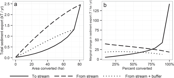
Figure 1. Theoretical landscape sediment export through each step of the simulation, in terms of (a) cumulative total export, in tons of sediment, and (b) marginal change in export, in tons of sediment per hectare converted per year (for kb = 2 and IC0 = 0.5; see figures S5 and S6 for effects of these and other model parameters on model behavior).
Download figure:
Standard image High-resolution imageIt is important to note that the C (cover) and P (practice) factors (which drive the differences in sediment export for different land-uses—see supplemental materials and Hamel et al 2015 for more detail) are quite similar for different natural land cover types; a greater difference is observed when comparing these factors for natural land cover (regardless of type) and agricultural land cover. For this reason, results similar to those outlined above are obtained for the conversion of other types of natural habitat (such as grassland) to agriculture, and not just forest conversion scenarios (table 2).
Table 2. Marginal sediment export (tons ha−1 yr−1), averaged across full simulation (conversion of entire landscape) and at 10% conversion of the landscape, for each of the conversion scenarios We show the marginal export at 10% conversion as an illustration of the early stages of expansion, which can be seen in figure 2 as the start of the line graph. See methods for description of theoretical, baseline and actual landscapes.
| To stream | From stream | From stream + buffer | Cropland | ||
|---|---|---|---|---|---|
| Average marginal sediment export (t ha−1 yr−1) for whole simulation | Theoretical (forest) | 30.1 | 30.1 | 17.6 | n/a |
| Theoretical (grassland) | 28.5 | 28.5 | 16.7 | n/a | |
| Iowa (baseline) | 2.9 | 3.2 | 2.2 | n/a | |
| Heilongjiang (baseline) | 6.3 | 7.5 | 5.0 | n/a | |
| Jiangxi (baseline) | 29.5 | 29.8 | 21.1 | n/a | |
| Mato Grosso (baseline) | 2.1 | 2.4 | 1.6 | n/a | |
| Iowa (actual) | 8.6 | 10.7 | 7.4 | 9.9 | |
| Heilongjiang (actual) | 10.3 | 14.0 | 9.1 | 13.9 | |
| Jiangxi (actual) | 29.0 | 39.0 | 24.5 | 37.8 | |
| Mato Grosso (actual) | 2.3 | 2.6 | 1.8 | 2.6 | |
| Marginal sediment export (t ha−1 yr−1) at 10% conversion | Theoretical (forest) | 5.2 | 39.8 | 18.5 | n/a |
| Theoretical (grassland) | 4.9 | 37.7 | 17.6 | n/a | |
| Iowa (baseline) | 1.1 | 5.5 | 2.7 | n/a | |
| Heilongjiang (baseline) | 4.1 | 6.3 | 3.9 | n/a | |
| Jiangxi (baseline) | 18.2 | 28.7 | 15.2 | n/a | |
| Mato Grosso (baseline) | 0.9 | 3.0 | 1.5 | n/a | |
| Iowa (actual) | 5.0 | 21.2 | 9.5 | 15.2 | |
| Heilongjiang (actual) | 5.9 | 15.0 | 8.0 | 5.2 | |
| Jiangxi (actual) | 16.8 | 43.6 | 17.9 | 8.2 | |
| Mato Grosso (actual) | 1.1 | 3.2 | 1.7 | 1.8 | |
3.2. Comparison of impacts across regions
The general trend seen in the theoretical landscape is preserved across all regions in the baseline and actual landscapes, despite differences in starting land-use configuration, as well as topography, erodibility and erosivity characteristic of a region. However, with the exception of Jiangxi, the average marginal sediment export for the real landscapes of the study regions is much lower than seen in the theoretical landscape, and the difference between scenarios is not quite as pronounced (table 2). For each hectare of habitat converted, Jiangxi exports on average more than ten times the sediment of Mato Grosso or Iowa, and four times that of Heilongjiang (figure 2).

Figure 2. Marginal sediment export for the baseline (a)–(d) and actual (e)–(h) landscapes for Iowa (a), (e), Heilongjiang (b), (f), Jiangxi (c), (g), and Mato Grosso (d), (h). Note the different scales for the y-axis. Because these models are uncalibrated these values should not be considered absolute, but the relative differences were consistent across other models and observations.
Download figure:
Standard image High-resolution imageThe differences in the average marginal sediment export (tons ha−1 for each step of conversion, averaged across the conversion of the entire landscape) belie the full differences between scenarios for most of the simulation, because the spike in sediment export in the final stages of conversion for the to stream scenario inflates the average. In all regions and for both baseline and actual landscapes, the marginal sediment export in the from stream scenario exceeds that of to stream for the first 80% of conversion, although the magnitude of the differences between scenarios is much greater in the actual landscapes than in the baseline landscapes (table 2, figure 2). Remarkably, for the first 15% of expansion in both landscape types, the from stream + buffer cuts sediment export per hectare in half compared to from stream.
In contrast to the baseline landscapes, differences between scenarios in the actual landscapes are enough to override the more general physical differences between regions. Despite the much higher average marginal sediment export for the conversion of the entire landscape in Jiangxi and (to a lesser extent) Heilongjiang compared to Iowa (table 2), agricultural expansion from stream in Iowa (figure 2(e), dashed line) causes higher marginal change sediment export in the first 10%–15% of conversion than agricultural expansion to stream or from stream + buffer in Jiangxi (figure 2(g), solid or dotted lines) and the first 60% and 40% of conversion for the same scenarios, respectively, in Heilongjiang (figure 2(f), solid or dotted lines). Furthermore, expansion from cropland in Iowa has a higher impact on sediment than the same scenario in either Jiangxi or Heilongjiang for the first 10% of conversion (figures 2(e)–(g); dash-dot line). This reversal in rankings of marginal sediment export reveals the potential for physical factors like climate, soil type and topography that characterize regions of high or low sediment export to be overwhelmed by the spatial configuration of land-use change.
3.3. Erosion potential across scenarios and regions
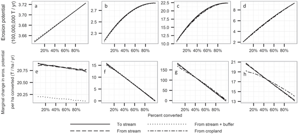
Erosion potential, the aspatial method for assessing sediment generation, shows little difference between the different land-use change scenarios (figure 3). This is because, unlike the spatially-explicit InVEST sediment model, erosion potential only uses a weighted-area average of land use factors in calculating the USLE. Though the spatial arrangement of how habitat is converted differs between scenarios, the overall amount of each habitat converted remains relatively constant (figure S4), and thus the impact of land-use is constant across all scenarios. There are dramatic differences between the regions in the amount of erosion potential, however, with Jiangxi having an order of magnitude higher values than the others (figure 3(c)). As increasingly more habitat is converted, the marginal erosion potential (change in erosion potential per hectare converted) declines in Jiangxi and Heilongjiang, and to a lesser degree in Mato Grosso (figure 3(f)–(h)). In contrast, the marginal erosion potential remains fairly constant in Iowa, irrespective of the amount of habitat remaining.
Figure 3. Erosion potential (T yr–1 for the entire watershed) (a)–(d) and marginal change in erosion potential per hectare converted (T ha–1 yr–1) (e)–(h) for Iowa (a), (e), Heilongjiang (b), (f), Jiangxi (c), (g) and Mato Grosso (d), (h).
Download figure:
Standard image High-resolution image
The difference in the shape of the response of erosion potential to conversion is a function of the difference in biophysical parameters for land-use between regions3 . As noted in 2.5, erosion potential values should not be compared directly with the potential soil loss predicted by InVEST (table 1), but their trends can be compared across regions and scenarios. Overall, the linear or smooth trends observed in figure 3 contrast with the highly non-linear trends in figure 2, confirming that spatially explicit methods are capable of more fully characterizing impacts within a landscape than aspatial methods such as erosion potential.
4. Discussion
4.1. Understanding the impact of the proximity to stream on sediment export
The impact of conversion to agriculture on sediment export is driven by a multiplicity of biophysical factors captured by the InVEST model. The simplified assumptions of the theoretical landscape allowed us to isolate the effect of land use from other drivers such as topography and initial land use configuration (figure 1). The convex shape (decreasing marginal change in sediment export) of the from stream and from stream + buffer scenarios results from the greatest impacts occurring in the early stages of conversion, when habitat nearest the stream is converted. In the from stream + buffer scenario, the effect is more nuanced because the process is attenuated by the riparian zone. The concave shape (increasing marginal change in sediment export) of the to stream scenario is a result of the pixels most important in providing the sediment retention service being converted last, therefore mitigating the impact of all converted upslope pixels (essentially acting as a continually shrinking buffer) until the final step of conversion.
The parameters tested in the theoretical landscape sensitivity analysis reveal some of the reasons for the lower or more variable marginal change in sediment export in real settings (see supplement). Slope and watershed extent (area) both affect the magnitude of the sediment export (figure S6). Therefore conversion from forest to agriculture of a pixel with either higher slope or greater contributing area will have a larger impact on sediment export. The simplified scenarios explored here in real landscapes show how much sediment export can change, depending upon how topography intersects with land-use at different distances from the stream.
4.2. Understanding the differences between regions
Most of the differences in the marginal change in sediment export between regions can be ascribed to the physical factors that characterize the basins. As noted in the model description, potential soil loss (as well as erosion potential) is a function of erosivity, erodibility and slope (R × K × LS). This is the amount of soil that is susceptible to erosion, with the land-management factors (C and P) held constant. Jiangxi ranks first in these factors of potential soil loss by a factor of 3–10 (table 1), driving the much higher average marginal sediment export in this region for both the actual and baseline landscapes.
Despite these general differences in sediment export between regions (i.e. due to physical factors), differences in sediment export between scenarios for each region are modified according to the location of land-use change in the region's watershed. Jiangxi and Heilongjiang both have much steeper slopes in the upper portions of their watersheds than other regions (and overall; table 1). Since these high-slope areas have such high levels of potential soil loss, they have a significant effect on sediment delivery even though they are located at points furthest from the stream. Agriculture in the Chinese regions is currently located on the areas of lowest potential soil loss, such that further agricultural expansion has a higher marginal impact in the actual than baseline landscapes. This is directly contrasted by Iowa, where all of the areas of high potential soil loss have already been converted to agriculture. However, in Iowa there is so little non-agricultural habitat remaining (<5%), mainly consolidated around the main streams, that all scenarios for the actual landscape can essentially be considered to be starting at the final steps of the to stream scenario of the baseline landscape. Therefore, the soil loss from remaining habitat conversion in Iowa occurs at a much higher marginal value than in its baseline landscape, and thus can exceed even the much higher physically-driven soil loss of Jiangxi.
4.3. Dealing with uncertainty
The InVEST model was not calibrated for this study (see supplement), which confers uncertainty in the absolute values of sediment export. Calibration parameters affect the magnitude of sediment export, and results based on absolute values should therefore be interpreted in the light of the uncertainties on calibration parameters. It is worth noting, however, that relative differences between scenarios appear to be less affected (figure S5). We verified the InVEST model predictions of sediment export by comparing them with empirical observations from the literature and with values from two peer-reviewed global sediment models, BQART and FSM (figure S7). We verified the lower and upper bounds (i.e. landscapes corresponding to 100% forest and 100% agriculture) to quantify the uncertainty on both the absolute and relative magnitude of predictions. Our model verification suggests that relative or at the very least rank order differences between sites hold, and that the relative increase in sediment export for each site (from a natural to an agricultural landscape) is credible. The model verification does not address uncertainties in model structure, in particular the expression for hydrologic connectivity. This modeling assumption drives the patterns observed in figure 1(a), and therefore the rates of change in figure 2. More research on hydrologic connectivity is needed to ascertain the precise shape of the curves. However, we note that the concept and its implementation for modeling is accepted by the hydrologic community (Borselli et al 2008, Bracken et al 2015). Importantly, the fact that a ten-fold difference in sediment loss can be reversed by the different patterns of habitat conversion explored here means that uncertainty in the pattern of future land-use is at least as important to consider for decisions as model calibration.
4.4. Why spatial context matters: the difference between erosion potential and sediment export
Although the marginal impact of each hectare of agricultural conversion on erosion potential is greater with more habitat in the landscape remaining, the marginal impact on sediment export to streams is the reverse, as long as the habitat converted is not that immediately adjacent to the stream. Because erosion potential does not account for habitat configuration and the buffering capacity of habitat downslope of a converted pixel, it not only overestimates the impact but misrepresents the relative impact between regions. For instance, Heilongjiang looks to be well below Iowa in marginal erosion potential (figure 3(b)), but its average marginal sediment export is higher than Iowa in every scenario (table 2). Similarly, Mato Grosso's marginal erosion potential is higher than Heilongjiang's and (for the first 20% of conversion) is on par with Iowa's, but average marginal sediment export is much lower in Mato Grosso than any other region. Finally, and most strikingly, Jiangxi is nearly an order of magnitude higher than Iowa in marginal erosion potential in the first 10% of conversion with no distinction between scenarios; from this information alone it would seem impossible that Iowa could actually exceed Jiangxi in marginal sediment export for the first 10% of the from cropland scenario.
There are two major differences between the erosion potential proxy for sedimentation and the InVEST sediment model. First, erosion potential only covers the source of the sediment, not its sinks. As already noted, decades of work have demonstrated the buffering capacity of habitat especially in the riparian zones (reviewed by Liu et al 2008, Yuan et al 2009). What is novel in this study is the illustration that order of magnitude differences in erosion potential can be overturned, depending on the configuration of land-use change. Second, the erosion potential methodology proposed by Saad et al (2013) is based on average measures of the physical factors characterizing a region (e.g., slope, climate, soil), rather than spatially-explicit combinations of these factors with land use-land cover. Indeed, authors noted that using average parameters representing broad biogeographic regions can result in estimates for erosion potential that 'may not be always comparable to results from local measurements and/or simulations performed on a site-specific area'.
4.5. What this means for decisions
If sourcing strategies and land management decisions are concerned with reducing impacts to water quality, general factors like soil erodibility, climate erosivity, and average slope that predict erosion potential for a region are important considerations. However, order of magnitude differences in erosion potential based on these factors alone (as seen between Jiangxi and Iowa) can be overridden by different spatial patterns of land conversion, specifically with regard to proximity to streams, regardless of natural habitat type. This means the specific configuration of land-use change should be considered when determining the final values of sediment exported to the stream because, for the same area of habitat converted, agricultural expansion further from the stream can compensate for a much higher erosion potential of a region. If a company were to select Iowa as the preferred choice for meeting increased soy demand through expansion, on the basis of erosion potential alone, they may have unwittingly selected the region of highest sediment export per hectare in the initial increments of agricultural expansion from current cropland.
The consistency of difference in sediment export between the from stream + buffer and from stream scenarios is remarkable, suggesting that relatively little habitat near the stream can perform a near-optimal sediment retention service for the same total amount of habitat converted. However, the resolution of the data (90 m) means that the buffer scenario should not be understood as a riparian buffer typical of agricultural best management practices, which may range from 5 to 10 m wide. Rather, it represents an absence of agriculture closest to the stream, and the model clearly demonstrates the effectiveness of such habitat configuration. Indeed, as suggested by the sudden threshold in the to stream scenarios at around 80% landscape conversion, after which point impacts increase much more steeply, it is likely that a much larger area would be required to buffer against the conversion of the entire watershed. There is also the additional consideration that cost of irrigation may increase with distance to stream, and the optimal placement for agriculture relative to streams will be determined by the trade-offs between operating costs of agriculture and social costs of the externalities of agricultural production. However, it is not the aim of this study to evaluate costs and benefits different best management practices in order to inform optimal placement, and the InVEST model is not designed (nor is current scientific understanding sufficient; Zhang et al 2009) to test the effectiveness of different buffer widths with varying upslope factors and configurations. Further, while buffers can prevent the siltation of reservoirs by keeping sediment out of the streams, the movement of soil from elsewhere in the watershed to the buffer zone could still be problematic for farming and other ecosystem services, especially when considering the fact that loss of topsoil is a major cause of reduced soil fertility. Nonetheless, this analysis has demonstrated the magnitude of difference possible in sediment export from maintaining habitat around streams and differences between landscapes not predicted with a non-spatially resolved method.
5. Conclusions
This study confirms the need to consider spatial assessment in improving land planning and decisions on agricultural expansion with respect to sedimentation and water quality. High erosion potential can be expected in landscapes with high erosivity (e.g. with intense rain events), high erodibility (e.g. silty soils), and high slopes. On the other hand, high hydrological connectivity will occur in areas close to the watercourse, or areas with low sediment retention capacity on the flow path to the watercourse (e.g. high slopes and/or bare soil). The actual change in water quality will depend upon the balance of the two.
Spatially-explicit yet still relatively simple process-based models like InVEST can provide valuable insights for decision-making and land management, beyond what can be gleaned from area-wide averages or proxies. Our work indicates that linearity of impacts cannot be assumed for land use change, and in the case of sediment export and impacts on water quality, non-linear effects are likely to be greatest in situations where: there is little remaining natural habitat; development is allowed within stream buffers; areas of lowest potential soil loss are already occupied; and/or hydrological connectivity is highly variable (land conversion will have a proportionally greater effect in areas with higher connectivity). When supply chain or other global prioritization decisions are being taken on agricultural development a spatially-explicit approach provides additional understanding of the broader implications of land-use change.
Acknowledgments
The authors wish to thank Peter Kareiva, Gretchen Daily, Henry King, Isabela Butnar, Edward Price, and Benjamin Bryant for advice and review of the manuscript that greatly improved its clarity. Unilever provided support to undertake this work.
Footnotes
- 3
The erosion potential for Jiangxi and Heilongjiang is nonlinear due to an artifact of the model; specifically that the P (practice) factor for cropland, obtained from the literature, is lower in these two regions. The P factor modulates the effect of the C (cover) factor, which is a measure of the sediment generation of each land-use type; a P factor closer to 1 means the land-use generates the full amount of sediment assigned by the C factor, while a P factor of 0.5 means the land-use only generates 50% of the sediment assigned by the C factor (Wischmeier and Smith 1978). The P factor for cropland in China is 0.5, whereas it is 0.8 and 0.9 for Mato Grosso and Iowa, respectively (see appendix in supplemental). Therefore, as the landscape becomes progressively more agricultural, C increases and P decreases, more sharply in the two Chinese sites. Because erosion potential is a linear function of the product of C and P, the opposite trends of these two factors results in the parabolic shape observed in 3a.