


ABSTRACT
We used daily full-disk Ca ii 854.2 nm magnetograms from the Synoptic Optical Long Term Investigations of the Sun (SOLIS) facility to study the chromospheric magnetic field from 2006 April through 2009 November. We determined and corrected previously unidentified zero offsets in the SOLIS magnetograms. By tracking the disk passages of stable unipolar regions, the measured net flux densities were found to systematically decrease from the disk center to the limb by a factor of about two. This decrease was modeled using a thin flux tube model with a difference in signal formation height between the center and limb sides. Comparison of photospheric and chromospheric observations shows that their differences are largely due to horizontal spreading of magnetic flux with increasing height. The north polar magnetic field decreased nearly linearly with time during our study period while the south polar field was nearly constant. We used the annual change in the viewing angle of the polar regions to estimate the radial and meridional components of the polar fields and found that the south polar fields were tilted away from the pole. Synoptic maps of the chromospheric radial flux density distribution were used as boundary conditions for extrapolation of the field from the chromosphere into the corona. A comparison of modeled and observed coronal hole boundaries and coronal streamer positions showed better agreement when using the chromospheric rather than the photospheric synoptic maps.
Export citation and abstract BibTeX RIS
1. INTRODUCTION
A long-standing goal of solar physics is to specify the time-varying distribution of magnetic flux on the solar surface. Aside from the intrinsic interest in learning about the creation and evolution of solar magnetic activity, such specifications are the essential boundary conditions for models and predictions of space weather and its impact on Earth. Achieving this goal is hampered by several observational factors. Measurements of magnetic flux density are usually limited to the line-of-sight (LOS) component (BLOS) and suffer from limited sensitivity, temporal and spatial resolution, and various instrumental biases. The projected apparent size of magnetic features shrinks approaching the limb, making them increasingly difficult to observe. Most measurements are made in the solar photosphere where the magnetic field is subject to dynamic pressure forces that complicate interpretations of the measurements and can even hide flux.
Daily full-disk observations of the chromospheric BLOS have been provided by the National Solar Observatory since 1996. These data have been used for some tentative studies with the main caveats being uncertainty about the quantitative conversion of circular polarization measurements in the core of the 854.2 nm line to BLOS, and various zero offsets. Most studies deal with qualitative differences between photospheric and chromospheric BLOS in specific features or in limited disk locations. Limited area observations of the chromospheric magnetic field have been available from several observatories for decades. For example, the Huairou Solar Observing Station observed photospheric and chromospheric quiet-Sun magnetograms near the solar disk center with equal spatial resolution; the observational results show similarities in the magnetograms and also in the temporal evolution of magnetic elements (Zhang & Zhang 2000). A series of comparisons of photospheric and chromospheric magnetic fields of active regions has been analyzed using longitudinal magnetic field measurements (e.g., Zhang et al. 1991; Zhang 1993a, 1993b) and vector magnetic field (Rüedi et al. 1995; Xu et al. 2010, 2012). Rüedi et al. (1996) presented the difference between the appearance of chromospheric and photospheric magnetic structures observed close to the solar limb due to the difference in height and projection effects. Yamamoto & Kusano (2012) recently combined chromospheric observations of BLOS with photospheric vector field measurements as a constraint in non-linear force-free field extrapolation into the corona.
Few studies have considered the global distribution of chromospheric BLOS in a synoptic context. Raouafi et al. (2007) studied the latitude distribution of polar magnetic flux elements in the chromosphere, and found two populations of flux elements in the polar region: the small ones are probably produced uniformly across the polar area, while the large ones result from the magnetic field of decaying active regions. Petrie & Patrikeeva (2009) found that the photospheric field is within about 12° being radial, while the chromospheric field has no strongly preferred direction, expanding in all directions to a significant degree.
In this study, we explore using BLOS measurements made in the solar chromosphere with the Ca ii 854.2 nm line as a way of specifying the large-scale flux distribution in a less constrained environment than the photosphere. Magnetic and gas pressure forces are more nearly equal in the chromosphere which allows long-lived flux features to be seen more easily near the limb (Figure 1). We emphasize the polar magnetic fields since they are difficult to observe in the photosphere and troublesome for the construction of global synoptic maps (e.g., Luhmann et al. 2009). Additionally, the transition between cycles 23 and 24 was unusual (e.g., de Toma 2012) and our work covers that period. We extrapolate the magnetic field from the chromosphere into the corona using synoptic maps of the chromospheric radial field distribution as a boundary condition.
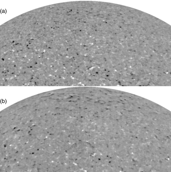
Figure 1. Northern quarter of the solar disk on 2008 June 29 showing observations of BLOS made with the core of the chromospheric 854.2 nm line of Ca ii (bottom) and with the photospheric 630.15 nm line of Fe i (top). Note the enhanced visibility of polar fields in the chromosphere. Photosphere and chromosphere displays saturate at ±50 and ±40 G, respectively.
Download figure:
Standard image High-resolution imageIn Section 2, we describe the observing instrument, data acquisition, and removal of signal offsets. In Section 3, we identify and track unipolar regions in chromospheric magnetograms and determine an empirical visibility correction function. In Section 4, we compare the chromospheric features with photospheric observations by SOLIS and the Solar Optical Telescope (SOT) on board Hinode. We also compare the empirical correction with that from a model based on the thin flux tube approximation. In Section 5, we show the polar field variations during the transition from solar cycles 23 to 24. In Section 6, we estimate the radial component of the chromospheric magnetic field based on various assumptions, construct synoptic maps of the radial component in the chromosphere, extrapolate the synoptic maps of chromospheric field and compare them with space data and the extrapolated photospheric field. In Section 7, we discuss and summarize these observation results.
2. OBSERVATIONS AND REDUCTION
Line-of-sight magnetic flux density measurements (BLOS) using the chromospheric Ca ii 854.2 nm line have been made occasionally since the 1970s (Harvey 2006) and daily full disk 854.2 nm BLOS mapping commenced at NSO/Kitt Peak in 1996. Starting in 2003, an instrument of the Synoptic Optical Long Term Investigations of the Sun (SOLIS) project, a vector spectromagnetograph (VSM; Keller et al. 2003), currently provides improved 854.2 nm measurements. The VSM instrument was upgraded with a better modulator of 854.2 nm circular polarization early in 2006 and with better cameras late in 2010. In this paper we use 740 good-quality observations from the stable period 2006 April 17 through 2009 November 27. We describe the data acquisition and reduction process in some detail because of issues that were neglected in previous uses of these data.
2.1. Instrument and Data Acquisition
The VSM is an equatorially-mounted, 50 cm modified Ritchey–Chrétien reflecting telescope that feeds a full solar disk image to a long-slit grating spectrograph. The full disk slit is oriented east–west in the sky and during our study period provided spectra with 1.125 arcsec spatial sampling and 4.1 pm spectral sampling. The full solar disk is scanned by moving the VSM in declination while tracking smoothly in right ascension. For the 854.2 nm observations, each 1.125 arcsec step consists of 64 modulated pairs of I+V and I − V dual beam spectra taken at the rate of 45.7 pairs s−1. A typical full disk observation consists of a dark image, a set of about 100 spectra that provides flat-field information, and a set of 2048 spectra obtained during the declination scan across the solar disk. The flat field spectra are contiguous scans of the solar image in right ascension. This scan starts with the telescope pointed a bit more than one diameter to the east and ends pointed similarly to the west. To the first order, each position along the slit is sequentially exposed to the same smeared slice of the solar image. These spectra are averaged and an instrumental intensity flat is obtained by fitting and removing the solar and telluric spectral lines. A magnetic field flat is obtained by applying the algorithm described next to the averaged I ± V spectra.
Reduction of the spectra to BLOS estimates was done by calculating three convolutions, stepped by one spectral pixel, of the first derivative of the I spectrum with I+V and I − V spectra. This is a small modification of the method described by Jones et al. (1992). The convolutions were restricted to a window of 148 pm full width centered on the 854.2 nm line. The wavelength difference of the zero crossings of the I ± V convolutions provides an estimate of the LOS magnetic flux density averaged over a spatial resolution element (BLOS). Noise level is about 3 G. The slit is curved with a radius of 16173 arcsec so that a geometric transformation of the slit positions is required to produce an undistorted solar image. Furthermore, two cameras are needed to capture the full east–west extent of the spectra and the separate spectra from these cameras are combined in the data reduction.
We used data from three distinct processing levels. Level 1 data are the full disk estimates of BLOS without any geometric corrections. Level 2 data have geometric corrections including a rotation of the images so that the Sun's rotation axis is parallel to the y coordinate axis. Level 2 includes subtraction of zero offsets based on the magnetic field flat. Level 3 data consist of mapping of each image into Carrington longitude and sine latitude coordinates. We used Level 2 and 3 data processed by a standard SOLIS pipeline and also wrote our own reduction codes starting with Level 1 data in order to apply corrections not included in the standard pipeline to get the best possible BLOS estimates and to create non-standard data products.
2.2. Removal of Zero Offsets
A LOS magnetic flux density of 1 G produces a circular polarization signal (V/I) of the order of 10−5 in the core of the 854.2 nm line. Such small signals may be systematically offset from zero by instrumental and reduction effects of similar magnitude. Even small zero offsets have major effects on extrapolations of surface magnetic fields and must be removed.
Individual Level 2 BLOS images may show zero offset streaks of a few gauss parallel to the scan direction. An example is seen in Figure 1(B). This offset is caused by imperfections of the magnetic flat field determined during the flat field scan. One source is that the portion of the Sun that is scanned during the flat may have a net non-zero BLOS. A second source is a slow position drift of the spectrum line relative to the flat field image that leads to signal streaks along the scan direction. The images also may show streaks parallel to the slit. These zero offsets are caused by noise in the camera readout electronics and also by atmospheric scintillation that changes the spectral intensity between alternate polarization states. These streaks are small scale and appear to introduce zero offsets that are uniformly distributed relative to a large-scale average. Thus they do not affect large-scale average determinations of zero offsets.
A second, systematic, zero offset appears when many standard pipeline Level 2 images are averaged. It is predominantly a center-to-limb variation. Investigation of this offset showed that it has an amplitude and sign that depend on position along the entrance slit. The cause is not clear but may be related to center-to-limb changes in the width, Doppler shift, and asymmetry of the core of the 854.2 nm line and perhaps weak polarization produced by the telescope. Because this offset is not radially symmetric it is a challenge to separate it from the polar fields near the solar limb. One advantage of the equatorial mounting of the SOLIS VSM is that the annual variation of the position angle of the solar rotation axis moves polar magnetic fields over a range of nearly 53° relative to the instrument scan direction. This helps to separate solar and instrumental signals.
The standard pipeline reduction does not correct either of these offsets so we applied corrections in our own reduction code. First, the center-to-limb offset was subtracted from our versions of Level 2 images. Then streak removal was applied to each position along the slit.
We used two methods to characterize the center-to-limb zero offset. Both methods involved construction and averaging of images restricted to selected ranges of the position angle of the solar rotation axis (P angle). In method 1 we used Level 2 full disk images interpolated to have a constant image diameter. Method 2 used our own reduction of Level 1 images to Level 2 but remapped the measurements onto a grid on which the x-axis is pixel position along the spectrograph slit and the y-axis is pixel distance from the limb. In both methods many individual images were created and averaged with several levels of rejection of extreme negative and positive values. In method 1 the rejection levels were 2, 3, and 4 standard deviations from the mean while method 2 used 5, 10, and 20 G. We found empirically that the difference between the averages with the least rejection and the most rejection appeared to leave most of the solar signal and remove most of the instrumental zero offset. So a zero offset image may be defined as Z = A2 − f(A3 − A1), where A1 is the average with the most rejection of extreme values, A3 is the average with the least rejection, A2 is the average with intermediate rejection, and f is an adjustable factor. In method 1 we used averages for eight P angle ranges and found that f = 2 gave good results. The median of these images rotated to a geocentric coordinate system produced a close approximation of the zero offset needed to correct Level 2 images. We reduced the remaining residuals of the solar signals by making an average of the image and a north–south flipped version with weights of 2 and 1, respectively. The final offset image is shown in Figure 2.
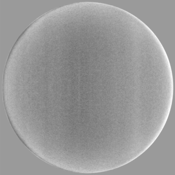
Figure 2. Best estimate of the average zero offset of a large number of Level 2 images. See the text for details. The range shown is ±2 G.
Download figure:
Standard image High-resolution imageSome streaks typically remain in a full-disk observation after removing the center-to-limb zero offset. The streaks are zero offsets that vary with position along the spectrograph slit. They are produced by small differences between the circular polarization flat image and individual spectra obtained during the full-disk scan and they change with each full-disk observation. We remove the streaks to the first order by subtracting an average of the BLOS image along the scan direction. The influence of real solar magnetic features on the average is minimized by excluding the solar poles (sine latitude outside the range ±0.8), values outside the range ±40 G, and then doing three iterations of the average calculation with values more than two standard deviations from the average excluded in each iteration step. After this average is subtracted the result is our best estimate of the true solar BLOS.
3. FLUX DENSITY VISIBILITY DETERMINATION
Because of the loss of resolution due to foreshortening and systematic vector orientations of flux elements, the photospheric and chromospheric LOS magnetic field near the solar limb generally becomes weaker and less visible than that at the solar disk center. We seek a function of distance from the disk center that compensates for this systematic reduced visibility, i.e., a visibility correction function. It is especially difficult to define such a correction for polar regions because we cannot observe the polar magnetic field over a large range of viewing angles. Generally speaking, the magnetic field in the photosphere is radial, and BLOS across the disk within an equatorial band varies as cos (ρ), the cosine of heliocentric angle (e.g., Svalgaard et al. 1978). However, the chromospheric field is more complex. Petrie & Patrikeeva (2009) investigated the low-latitude chromospheric field and found that it has no strongly preferred direction, expanding in all directions to a significant degree. Therefore, the cosine equation does not fit the variation of the chromospheric LOS flux density moving across the disk. Furthermore, from Figure 1, we also see that close to the solar limb, the magnetic field in the chromosphere is stronger than in the photosphere, while close to the solar disk center the opposite is true. This further demonstrates that as the magnetic field moves from the solar limb to the solar disk center, the photospheric and chromospheric fields cannot have the same variational function. Therefore, a fit function to describe the center-to-limb variation of the chromospheric LOS flux density is needed.
Here, we assume that BLOS features in the poles and east–west limb regions follow the same visibility function and that the magnetic flux properties of equatorial unipolar regions and polar regions are similar. We track unipolar regions near the equator as they move across the solar disk to find how the chromospheric magnetic fields observed close to solar limb relate to observations near solar disk center. We use Level 3 data to identify and track unipolar regions close to the solar equator. High-latitude regions are excluded because they do not pass close to disk center and their boundaries change significantly during a disk passage. For each identified unipolar region (typically the decaying remnants of old active regions that cover tens of degrees and evolve slowly), we construct an encompassing rectangular outline in longitude and sine latitude that tracks the region at the Carrington rotation rate, and utilize all of its daily observations from its appearance near the east limb to its disappearance near the west limb. We do not use regions for which daily observations are sparse or noisy.
We selected 20 unipolar regions, and tracked them from the east limb to the west limb. The unsigned magnetic flux density in these regions is larger than 8 G and the ratio of magnetic flux in the major polarity to the minor polarity is higher than 3. As the unipolar region moves across the solar disk center, we compute the distance, r, from the solar disk center of each pixel in the unipolar region, and analyze the distribution of magnetic field as a function of r. We only include pixels with magnetic field larger than 4 G (i.e., above the 3 G noise level). The distributions of magnetic field as a function of r are fitted with a second-degree least-squares polynomial and a visibility correction function for each unipolar region is obtained by inverting the polynomial functions.
We average the visibility correction functions for all unipolar regions, and then fit an overall correction factor for the LOS field in the chromosphere. The final visibility correction function, fcor, is obtained by fitting the averaged correction factor by a polynomial function:
where r is the ratio of the pixel distance from the solar disk center to the solar radius. Because the full-disk measurements consist of observations made with two cameras, the correction factors for the cameras are fitted separately, as shown in Figure 3. In this figure, we see that there is only a small difference in the visibility correction factors at the west and east limbs due to the different cameras and slow evolution of the unipolar regions. For practical purposes, especially near the poles, we use only the even order terms in r of fcor and ignore the small odd order terms.
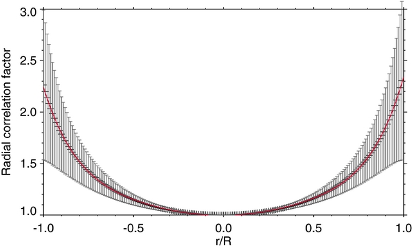
Figure 3. Visibility correction function of BLOS observed with the chromospheric 854.2 nm line of Ca ii. The heavy red line is the polynomial fit for the correction factor. The gray bars represent one standard deviation of the average correction factor. Separate fits were made for the east (left) and west (right) magnetograms. R is the solar radius.
Download figure:
Standard image High-resolution image4. COMPARISON OF 8542 FEATURES WITH MODELS AND PHOTOSPHERIC OBSERVATIONS
In this section, we examine individual polar magnetic features observed in the chromosphere and photosphere to study how their appearance changes with height. We also compare observations with a model based on the thin flux tube approximation for further insight to the visibility correction function determined in Section 3.
4.1. Polar Fields as Observed by Different Instruments
As shown in Figure 1, the network polar fields in the chromosphere are easier to observe than in the photosphere. Raouafi et al. (2007) and Petrie & Patrikeeva (2009) pointed out that network magnetic features close to limb appear stronger in the chromosphere than in the photosphere. One reason for this is that the spreading canopy fields are easier to observe in BLOS observations of the chromosphere. Another reason is the ubiquitous, dynamic horizontal fields in the photosphere near the limb (Harvey et al. 2007; Lites et al. 2008) produce random background noise that, unless averaged in time and/or space, overwhelms the long-lived network fields. This noisy background is much smaller in the chromosphere. In this study, we compare the magnetic features seen in the VSM chromospheric observations with VSM photospheric observations as well as high spatial resolution Hinode observations.
We compare the south polar region of a chromospheric VSM magnetogram with a photospheric VSM magnetogram. Nearly simultaneous Ca ii 854.2 (lower right panel) and Fe i 630.2 (top right panel) VSM observations are shown in Figure 4. For the dominant positive polarity, the chromospheric observation shows more magnetic network features than the photospheric magnetogram. These features are stronger in the chromosphere than in the photosphere. The photospheric magnetogram is dominated by the random horizontal intranetwork fields close to the limb and barely shows network fields there. The average magnetic flux density of the major polarity in the region is 4.6 G in the chromosphere, which is significantly stronger than 3.7 G in the photosphere. This is consistent with the results of Petrie & Patrikeeva (2009). The magnetic features in the chromosphere appear more diffuse than in the photosphere.
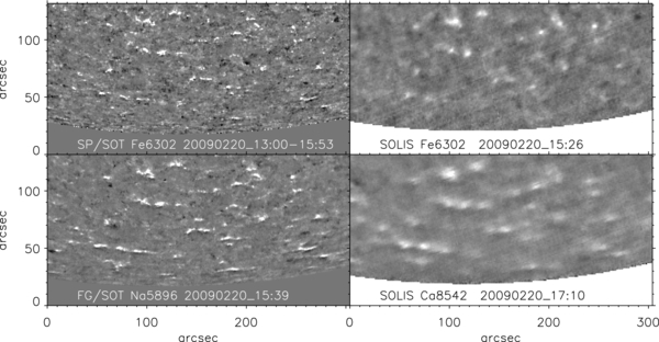
Figure 4. Nearly simultaneous south pole BLOS observations with the pole tipped toward Earth by 7 04. Left: Hinode observations. Right: VSM observations. The top row shows photospheric (630.2 nm) observations and the bottom row shows low and mid chromosphere observations. White represents the fields directed toward the observer and black away. The dominant polarity in this polar region is light that corresponds to a field directed outward from the Sun. VSM and SP observations saturate at ±30 G, and FG observation saturates at ±0.006 IC in circular polarization.
Download figure:
Standard image High-resolution imageWe also compare the VSM observations with nearly simultaneous Hinode Narrowband Filter Imager (NFI) data taken in the Na i D passband at −16 mÅ from the Na i D line core. Since NFI provides images at a high spatial sampling of 0 16, finer features are observed (lower left panel in Figure 4) than in the VSM observations. Although the Na i D line is often taken to be chromospheric, Leenaarts et al. (2010) found that most Na i D brightness is not chromospheric, but instead samples the magnetic concentrations that make up the quiet-Sun network in the photosphere well below the height where they merge into chromospheric canopies. Nevertheless, magnetic canopies are clearly visible in the magnetogram. These magnetic canopies are not as obvious in the chromospheric VSM observation although almost all of the strong magnetic features of majority polarity seen in the Na i D line observation appear in the VSM chromospheric magnetogram. The differences in the appearance of canopies in the Na i D and VSM Ca ii 854.2 nm magnetograms can be partially attributed to differences in spatial resolution. The differences may also be partly due to differences in the measurements themselves: NFI is a filter-based measurement of the circular polarization signal in a given (narrow) wavelength passband while the VSM measurements are the LOS flux in G derived from spectrally well-resolved Stokes I and V profiles using the weak-field approximation. The NFI signal strength and sign may be affected by unknown Doppler shifts of the polarized line profile.
In contrast, the VSM photospheric magnetogram is more similar to the 4.8 s exposure time Hinode Spectro-Polarimeter (SP) magnetogram. This is to be expected since the two instruments observe the same spectral line and, thus, sample the same height in the atmosphere. With the improved spatial resolution, the magnetic flux density measured by SP in the polar region is higher; the average positive field is 5.8 G in the SP observation compared to 3.7 G measured by VSM using the same spectral line.
4.2. Comparison of Observations with a Flux Tube Model
Here we investigate if there is a plausible way to explain the empirical visibility correction function using a specific flux tube model. There may be many ways to model the function and here we only examine one of the most simple possibilities. For convenience we use a numerical flux tube model based on the thin flux tube approximation. Previous works (e.g., Grossmann-Doerth et al. 1988; Bruls & Solanki 1995; Solanki et al. 1999; Yelles Chaouche et al. 2009; Pietarila et al. 2010) have found that the expansion of magnetic fields with height in the photosphere is consistent with the thin flux tube approximation (Roberts & Webb 1978; Defouw 1976). Here we wish to see if this is also true in the higher layers sampled by the Ca ii 854.2 line core magnetograms. To study this, we constructed two-dimensional flux tube models (0th order in radius for the vertical magnetic field and 1st order for the radial magnetic field) using the SRPM model of the quiet-Sun low chromosphere (Fontenla et al. 2007) as the external, non-magnetic model and the FALP network model (Fontenla et al. 2006) as the magnetic flux tube interior model. To compute the Wilson depression and magnetic field vector, we need to specify the tube radius, r0, and field strength, B0, at z = 0 km. We made two models, one with B0 = 1300 G and r0 = 400 km and the other with B0 = 1400 G and r0 = 600 km. Note that the thin flux tube approximation is strictly valid only when the flux tube radius is smaller than the gas pressure or density scale heights, i.e., both of the constructed models are outside the strict validity range of the approximation but that is not significant for this exploration. As shown in Pietarila et al. (2010), the choice of r0, and to lesser extent B0, are the main factors for the expansion, while the choice of the flux tube interior atmospheric model plays in comparison an insignificant role.
We computed BLOS from the two models at various viewing angles and determined the visibility correction function (B(cos (0))/B(cos (θ))). Shown in Figure 5 is the visibility correction from the models at two different heights, 330 km (well below the formation height of the Ca ii 854.2 magnetograms) and at 770 km (low to mid chromosphere where the bulk of the Ca ii 854.2 magnetogram signal likely originates from). The green lines in the bottom panels show the visibility correction function for when the field is sampled at a uniform height through the cross section of the tube. They are the same as a purely radial correction, cos (θ), at both heights and for both models: the model-based visibility correction is not in agreement with the empirical correction (shown in the black solid line).
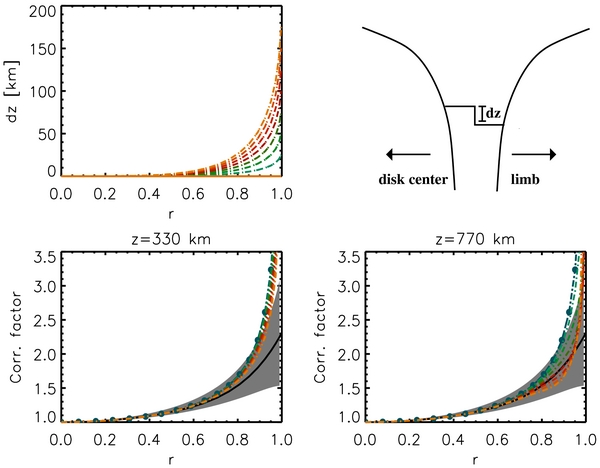
Figure 5. Visibility correction functions based on thin flux tube models. Top left: dz as a function of solar radius for the different models. Top right: schematic depicting dz. Bottom: visibility correction functions from the models at z = 330 km (left) and 770 km (right). The colors are the same as in the top left plot. The dashed line is for a flux tube model with B0 = 1300 G and r0 = 400 km and dash-dotted line for B0 = 1400 G and r0 = 600 km. The black solid line and gray shading show the empirical visibility correction and its uncertainty.
Download figure:
Standard image High-resolution imageThe discrepancy can be removed if we consider the center-to-limb variation of the signal formation height inside the flux tube. Off disk center the optical depth scale changes asymmetrically across the flux tube: due to the reduced density and opacity inside the flux tube, the optical scale of rays passing through the tube is stretched relative to rays not traversing the tube. This leads to the optical depth unity being lower in the atmosphere on the limb- than the center-side of the flux tube when the viewing angle is non-radial. To approximate this effect, we divided the flux tube in two at the tube center and imposed a formation height difference, dz, between the two halves (see the schematic in the top right panel of Figure 5). The center-side half is still sampled at 330 km or 770 km, while the limb-side half is sampled at a lower height, z−dz. The center-to-limb variation of dz was constructed to be zero at and near disk center and to increase strongly toward the limb (top left panel in Figure 5). We tested different amounts of dz (shown in different colors in the top left panel).
The visibility correction functions determined from the models with dz ≠ 0 (bottom panels) are in better agreement with the empirically determined visibility correction at z = 770 km. As dz increases the correction begins to flatten out near the limb resembling the behavior of the empirical correction. The visibility correction for z = 330 km does not change significantly and is still consistent with the photospheric field being mostly radial.
By introducing an asymmetry in the formation height of the signal, lower on the limb-side than on the disk center-side, the flux tube model at z = 770 km mimics the empirical correction satisfactorily until very near (r = 0.95 rSun) the limb where it begins to increase too fast (and where the empirical function is poorly determined). In general, however, the corrections vary significantly with height. For example, higher up in the atmosphere (not shown) the effect of introducing dz is the opposite: the visibility correction becomes steeper than the cos (θ) function. Based on the simple approach used here, we can conclude that the flux tube model agrees reasonably well with the empirical function for a specific height and set of parameters but varies strongly depending on which height in the chromosphere is considered and is therefore very model-dependent. Future work will need to consider more realistic models.
5. POLAR FIELD VARIATIONS 2006–2009
The transition between cycles 23 and 24 was very unusual: there was an unusually large number of days without sunspots and the polar magnetic fields were relatively weak. Magnetic activity during the years 2006–2009 was very weak with sunspot numbers reaching the lowest values in about 100 years (de Toma et al. 2010). Also the amount of spotless days reached above 80%. The polar field in the photosphere during the unusual minimum was roughly 40% weaker than the previous three minima (Kirk et al. 2009; Schrijver & Liu 2008; Sheeley 2008; Svalgaard & Cliver 2007; Wang et al. 2009). To the best of our knowledge, only Petrie (2012) has investigated the behavior of the chromospheric magnetic field during the unusual transition. He prepared butterfly diagrams of chromospheric measurements and showed that the latitude centroids of active region fields behaved differently compared to those in the photosphere. Since he used data that was not corrected for zero offsets or the radial visibility function, it is useful to see if there are any changes that can be attributed to the corrections we applied to the same data set. In particular, we want to determine how well the visibility correction function removes changes in the corrected polar field measurements caused by the annual variation of the Bo angle.
We apply the visibility correction to Level 3 daily maps and average the signal over a latitude range of 60° to 90° and ±40° from the central meridian. The results are shown in Figure 6(A). Aside from a residual annual variation, the south polar average of 4 G does not change significantly over the 3(1/2) year period. The north polar average changes from about −5 G to near zero over the same time period. These observations agree with some photospheric measurements that also show a nearly constant south polar field and a weakening north polar field. It is also obvious that the changing Bo angle causes annual changes in the observed fluxes in the sense that the polar signal is stronger when the pole is more visible. This suggests that the visibility correction function is too small near the limb. However, Figures 6(B) and (C) show that the annual variation is confined to the majority polarity at each pole with no significant variation of the minority polarity. The annual variation of the majority polarity is more obvious in the north pole than in the south pole. We found that sensitivity to the changing Bo angle can be switched between the major and minor polarities by small changes to the zero offset corrections. Finally, Raouafi et al. (2007) noted that large concentrations of chromospheric polar magnetic flux were distributed less uniformly near the poles than smaller concentrations. If larger concentrations are predominantly the major polarity and smaller ones the minor polarity, this may help explain the different time behaviors of the majority and minority fluxes, which perhaps helps to understand the source of polar field.
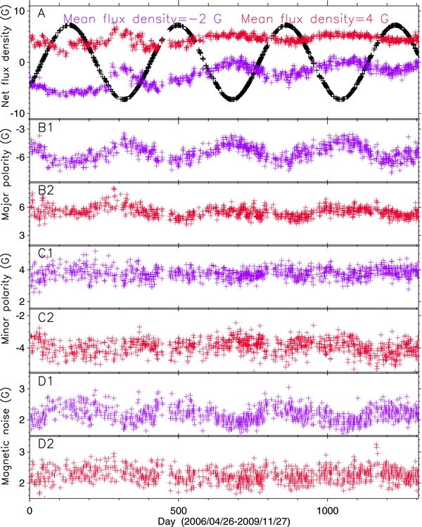
Figure 6. Time variation of the average polar LOS magnetic flux density. Each symbol represents one daily observation that has been corrected for the visibility function and averaged over a latitude range from 60° to 90° and a central meridian distance ±40°. The red (purple) symbols are the south (north) pole. The black symbols are the latitude of the sub-Earth point. (A) Averages of measurements without regard to sign. (B) Averages of measurements restricted to the sign of the majority polarity at each pole. (C) Averages of measurements restricted to the minority polarity at each pole. (D) Standard deviation of the averages in (A).
Download figure:
Standard image High-resolution imageWe examine this complicated situation in more detail by constructing partial butterfly diagrams as shown in Figure 7. Here we see that the sensitivity to the changing Bo angle is present at all latitudes in the polar regions. We also see the steady weakening of the north polar flux density. We note that our diagrams agree well with the more extensive ones presented by Petrie (2012).
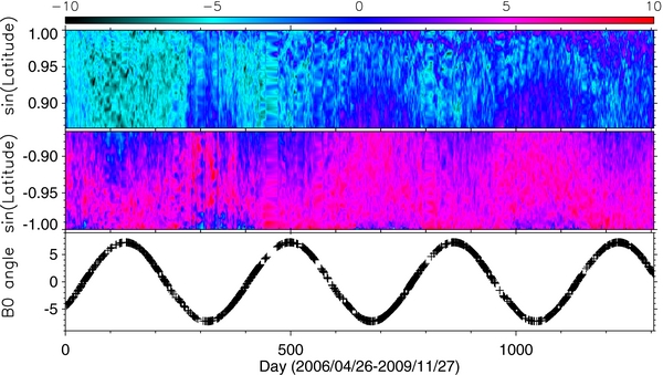
Figure 7. Time variation of the daily average polar chromospheric LOS magnetic flux density vs. sine of the latitude. Each pixel is the averaged LOS flux density over a central meridian distance of ±40 deg after correction for the visibility function. The bottom panel shows the latitude of the sub-Earth point. Data gaps have been filled by linear interpolation. The color bar scale is in G.
Download figure:
Standard image High-resolution imageWhy does the visibility correction function determined from the disk passage of unipolar regions fail to remove the Bo angle sensitivity? One explanation is that the zero offset correction near the limb is wrong. In this case a false zero offset, corrected by the visibility function, would show an annual variation. However, all polar latitudes show the annual variation and the zero offset appears to be large only close to the limb (see Figure 2). Another possibility is that the distribution of field inclinations to the radial direction is systematically different in low-latitude unipolar regions compared with unipolar polar regions. Or the major and minor polarity patches may have different distributions of field inclinations to the radial direction. Our assumption that quasi-unipolar regions at both low latitudes and in polar regions are similar may be too simple.
One robust result is that the north polar average flux density was decreasing nearly linearly with time by a factor of about three during our study period. The south polar average flux density was nearly constant until Fall 2009 when it started to decrease. In the next section, we take advantage of the annual variation of the Bo angle to help understand the polar fields.
6. EXTRAPOLATION OF CHROMOSPHERIC MAGNETIC FLUX DISTRIBUTION
We use the corrected chromospheric BLOS measurements as boundary values for extrapolations of the global magnetic field into the corona. Such extrapolations have been done for more than 40 years using photospheric measurements. As far as we know, this is the first time that global chromospheric measurements have been used.
The magnetic field at the solar surface can be readily extrapolated into the corona if the field is current free, in which case it satisfies Laplace's potential field equation. The observed magnetic field provides the boundary condition. Following Chapman (1943) the surface field can be represented as a set of magnetic poles. This pole method was first used by Schatten et al. (1969) to calculate the global coronal magnetic field from BLOS observations using an addition of a spherical source surface outer boundary condition above which field lines are constrained to be radial. This was the first potential field source surface (PFSS) model. Newkirk et al. (1968) did not use an outer source surface and treated the BLOS observations not as poles but as components of a field that is radial at the photosphere. Altschuler & Newkirk (1969) replaced the radial method by one in which BLOS measurements are directly used to constrain a finite series of Legendre polynomial spherical harmonic coefficients from which the potential field can be computed. This LOS method became popular and numerous improvements were made (e.g., Adams & Pneuman 1976; Riesebieter & Neubauer 1979; Hoeksema 1984; Zhao & Hoeksema 1993; Rudenko 2001). The LOS method was persuasively criticized by Wang & Sheeley (1992) who noted that the solar magnetic field in the photosphere is nearly radial and therefore nonpotential. They resurrected the radial method, this time with a source surface, and showed that using the assumption that the magnetic field in the photosphere is radial to correct BLOS measurements produced better agreement with a variety of observations. This radial method has prevailed for PFSS extrapolations in recent years (e.g., Luhmann et al. 2002), though not without some concerns (e.g., Rudenko 2004). Recently, Tóth et al. (2011) demonstrated that naive use of a high-degree spherical harmonic expansion to represent the potential field can lead to serious errors, especially near the poles. In spite of these issues, BLOS measurements have been combined into synoptic maps of the entire solar surface flux distribution and these maps have been used to infer the structure and dynamics of the solar corona and heliosphere with considerable success.
In the case of chromospheric BLOS measurements, as noted by Petrie & Patrikeeva (2009), there may be very significant advantages in returning to the old LOS PFSS method rather than using the radial method. This is because the chromospheric field should be closer to a force-free, current-free state and it has substantial non-radial components. Because of the prevailing use of the radial method and the availability of extrapolation codes, for this exploration we construct synoptic maps of the estimated radial component of the chromospheric magnetic flux distribution. We made only diachronic (over a range of time) maps constructed from enough daily observations to cover single solar rotations. Thus, none of our maps are intended to be synchronic, i.e., representing the entire solar surface at a given instant of time.
6.1. Estimating Radial Magnetic Flux Density
In principle one can use the changing perspective provided by solar rotation over several days to resolve a series of observations of BLOS into radial, and two horizontal components. The major assumption is that the magnetic field vector at each point on the solar surface does not change as the Sun rotates. This technique has a long history in studies of velocity and magnetic field vectors in sunspots (e.g., Cowling 1946; Plaskett 1952; Kinman 1952; Adam 1963; Harvey 1969). It was first used to study large scale solar magnetic fields by Howard (1974) and Duvall et al. (1979), and subsequently by many others. Global synoptic maps based on this method have been made by Grigoryev et al. (1986), Grigor'ev & Latushko (1992), Pevtsov & Latushko (2000), Ulrich et al. (2002), Wang & Zhang (2010), and Mordvinov et al. (2012). Such synoptic maps have also been combined over long time periods to construct butterfly diagrams of the components of the magnetic field (e.g., Ulrich & Boyden 2005; Vecchio et al. 2012; Mordvinov et al. 2012; Ulrich & Tran 2013). We attempted to use this method with our chromospheric measurements but were unable to get good solutions for all three vector components due to noise, evolution of the magnetic field vector, and the small change of Earth's heliocentric latitude during one rotation. However, we were able to get good solutions for just the zonal and meridional plane components (cf. Ulrich et al. 2002). This prompted a rather complicated method to estimate the global distribution of chromospheric radial magnetic flux density.
Briefly summarized, we start with a Carrington rotation map of the meridional plane component of the chromospheric magnetic flux density. At low to moderate latitudes the meridional component is dominated by the radial component but at polar latitudes the north–south component becomes increasingly significant. To suppress the north–south component, we average the meridional component over all longitudes and subtract the averages from the map as a function of latitude. The change in the map is minor at small latitudes but major at polar latitudes. Then we add an estimate of an annual running average of the radial component of the flux density as a function of latitude. The result is a hybrid map approximation of the radial flux density distribution. The longitudinally-averaged values of the map are based on a 365-day average of the radial component while the other details of the map are predominantly the radial component determined from one Carrington rotation of observations near the central meridian. We note that Ulrich & Tran (2013) developed a different method of separating the radial and north–south components of the near polar photospheric magnetic fields by deducing the long-term average tilt of the fields at high latitudes.
A Carrington rotation map of the meridional plane component of flux density can be built from data taken during a solar rotation in at least two ways. BLOS along the central meridian is the meridional plane component of the full vector field. So the simplest way to make the map is to merge data onto a Carrington rotation coordinate grid from a series of daily observations restricted to a small range of distance from the central meridian. This classic type of map has been used for photospheric observations since the 1960s. The zonal (east–west) component of flux density is suppressed by restricting observations to those made near the central meridian. A more complicated way, in principle making better use of the observations, is the vector resolution method described above. We used both methods to construct maps of the meridional component of flux density for five selected Carrington rotations. Both methods produced nearly identical maps and we use the results of the second method in what follows (see Figure 8). The input data are Level 3 daily maps that have been corrected for zero offsets and the visibility correction function. Then we subtract the longitudinally-averaged meridional flux at each latitude. This is done with three iterations, successively rejecting values in excess of two standard deviations from each average. The result is a map with zero average meridional component as a function of latitude (see Figure 8, middle).
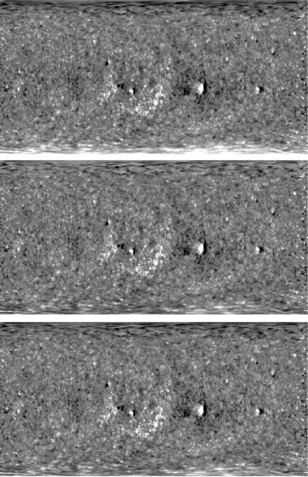
Figure 8. Three synoptic maps of Carrington rotation 2062 showing chromospheric magnetic flux density from −13 to 13 G. Abscissa is the Carrington longitude from 0 to 360 deg. Ordinates are sine latitude from −1 to 1. The upper panel is the meridional plane component. Note the strong signal near the south pole. The middle panel is the same minus the average of each latitude row. The lower panel is the middle map plus the average radial component at each latitude based on a 365-day data set. Note the nearly equally strong poles. See the text for details.
Download figure:
Standard image High-resolution imageNext, we estimate running 365-day averages of the radial and north–south components of the chromospheric magnetic flux density. Input data are daily Level 3 maps of BLOS that have been corrected for zero offsets but not for the visibility correction function (using the visibility correction function removes variations that allow the radial and north–south components to be separated). First, we make averages of the available observations for a series of Carrington rotations. Data covering a period of 38 days centered on the middle time of the Carrington rotation are used to ensure complete coverage of the slowly rotating poles. BLOS values in excess of ±20 G are excluded in the averaging as are locations with fewer than three measurements from the original full-resolution observation. Then, from each Carrington rotation average, we average the values that are within ±30° from the central meridian in order to suppress east–west flux components. One year of these data centered on the mid-time of a Carrington rotation are resolved into radial and north–south components as a function of latitude by means of least-squares fitting. The equation of condition is BLOS = Bradial(cos (b)cos (Bo) + sin (b)sin (Bo)) + Bnorth-south(sin (b)cos (Bo) − cos (b)sin (Bo)), where b is latitude and Bo is the latitude of the sub-Earth point. The process is repeated for all available Carrington rotations. The resulting time series of the radial component of the chromospheric flux as a function of latitude is noisy. We fit each time sample using a fifth-order cubic spline in sine latitude over the range ±0.97 and then in time with a linear function at each latitude. A final estimate of the radial component map is the sum of the fit just described and the map produced as described in the previous paragraph for a selected Carrington rotation (see Figure 8 bottom).
With both the radial and north–south components of the field now separated, it is straightforward to estimate the systematic tilt of the field relative to the radial direction. We find that the south polar field was systematically tilted away from the pole during our study period while the north polar field is more nearly radial. This finding is also evident in Figure 8 by comparing the upper and lower panels, which show little change in the north polar region compared to the south polar area.
6.2. Results of Extrapolations
The Global Oscillations Network Group (GONG) project produces full disk photospheric BLOS magnetograms once per minute and these are used as boundary conditions for a PFSS model between 1 and 2.5 solar radii (Petrie et al. 2008) using source code described by Luhmann et al. (2002). We compare PFSS results from GONG observations for selected Carrington rotations (http://gong.nso.edu/data/magmap) and PFSS results produced by using our estimated chromospheric radial flux synoptic maps as input data to the model. Note that the GONG data we used is not fully corrected for zero offsets, which may slightly degrade the quality of its extrapolated fields. We used GONG rather than another photospheric data source because we could use exactly the same extrapolation code on both the photospheric and chromospheric observations. Coronal holes are sensitive indicators of open field lines near the solar surface and, with care (see Robbrecht & Wang 2012), the equatorial coronal streamer belt indicates the position of the boundary at the upper surface of the model that separates opposite hemispheric polarities (polarity inversion or neutral line). Ideally our extrapolated flux map results would show agreement between the observed and predicted coronal hole boundaries and also the observed streamer and neutral line positions.
We use STEREO/SECCHI Carrington synoptic maps (http://secchi.nrl.navy.mil/synomaps) of the corona at 2.2 solar radii to make an estimate of the streamer positions, and also a composite of central meridian maps using 304 and 171 Å data to estimate coronal hole boundaries. The 304 maps are good for polar hole boundaries (minimum coronal obscuration) while the 171 maps are more sensitive for non-polar holes. Typically there are four streamer maps for each Carrington rotation: two from each spacecraft and two from each limb. We fill gaps and noisy locations with a high-order cubic spline fit to the good parts of each map and then average the maps to make the streamer estimate. To make the coronal hole boundary map, we average the maps from both spacecraft for each wavelength, reduce the original resolution to match that of our model results by block averaging and then apply a 5 × 5 median operator. A threshold is found that separates coronal holes from the rest of the Sun and a binary mask is produced for each wavelength. The masks are combined by using the "or" operator and spurious tiny features removed by manual editing. A few non-coronal hole features remain in the maps. The coronal hole boundary is drawn by using a Laplacian operator. This process produces coronal hole boundary and streamer position maps that are averaged over a time period similar to that covered by the magnetic synoptic maps.
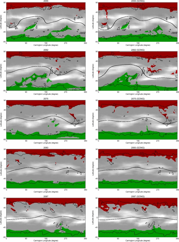
Figure 9 shows the comparison of streamer/neutral line and coronal hole boundaries for the chromospheric and photospheric (GONG) extrapolations. The observed streamer and coronal hole boundary information is identical for the chromosphere and photosphere maps. It is the model coronal hole boundaries and the neutral line positions that differ. The polar coronal hole boundaries are systematically too close to the equator in the photospheric maps, especially in later Carrington rotations. The chromospheric maps show better polar coronal hole boundary agreement. Spurious equatorward extensions from the model polar holes are seen in all the photospheric maps, especially in the north. The chromospheric maps show such doubtful extensions only in the south of rotations 2062 and 2083. Model holes not attached to the poles in both maps tend to match poorly in position and area with the observed features. The model holes are often too far from the equator and are either too small or too large in area. The photospheric holes are systematically larger than the chromospheric ones. Summarizing the coronal hole agreements, we see that the chromospheric extrapolation matches the total hole area better than the too-large photospheric hole boundaries. In other words, the photospheric extrapolation has more area of open field lines than the chromospheric one.
Figure 9. Five pairs of maps for selected Carrington rotations. The left column includes coronal hole locations (green and red colored areas) and a neutral line at 2.5 solar radii (smooth line near the equator) based on extrapolations of chromospheric measurements. The right column is that same for extrapolated photospheric (GONG) measurements. The gray-scale image is streamer locations from STEREO/SECCHI observations at 2.2 solar radii. The irregular line indicates coronal hole boundaries estimated from STEREO/SECCHI observations using 171 and 304 Å wavelengths.
Download figure:
Standard image High-resolution image
Turning to the streamer/neutral line comparison, we note a general failure of either extrapolated neutral line to show enough latitude excursion to match the observed streamers. The chromospheric neutral line shows a tendency to be north of the actual streamer band (especially rotation 2075). Generally, the photospheric and chromospheric neutral lines agree better with each other than they do with the streamers. An exception is rotation 2062 where the chromosphere extrapolation agrees better with observations on the left (east) while it seems that the photosphere extrapolation might agree better on the right (west). Robbrecht & Wang (2012) show similar maps for rotations 2061 and 2075. Our neutral lines for these rotations show similar shapes to theirs but for both the photosphere and chromosphere our neutral lines seem to be displaced slightly northward giving a poorer match to the observed streamer band.
7. DISCUSSION AND SUMMARY
Observations of the chromospheric magnetic field offer an opportunity to get a more complete view of the global solar magnetic flux distribution. We explored ways of utilizing this potential with 3(1/2) years of daily full-disk observations of BLOS from the core of the Ca ii 854.2 nm line.
Instrumentally, we found a zero offset that had not been previously known and devised a way of removing it. Separating this offset from solar polar magnetic fields was enabled by the large annual variation of the position angle of the solar rotation axis. It will be necessary to repeat the offset analysis for post-2009 observations since a new reduction method for 854.2 nm and new cameras were installed.
The center-to-limb visibility of foreshortening-corrected chromospheric BLOS was studied by tracking the disk passage of stable, quasi-unipolar regions. We found it to vary much less than the photospheric BLOS. This result confirms and extends previous work by Raouafi et al. (2007) and Petrie & Patrikeeva (2009). The cause for the smaller variation is a widening of the distribution of field inclination angles from radial with increasing height within magnetic flux elements (magnetic canopy). There is a lot of variance in the visibility, which suggests that different quasi-unipolar regions may have different inclination distributions. Observations of the chromospheric BLOS at the north and south polar regions support this suggestion. The visibility of the fringed canopy field was quite different at the two poles during our study period: the south readily showed canopies while they were much less visible in the north. Some of these results can be explained if the south polar fields are systematically tilted away from the pole more than in the north, as seen in Figure 8 of Feng et al. (2009) based on stereoscopic reconstructions of 2007 observations, and supported by our separation of radial and north–south components of the polar fields. This super-radial chromospheric expansion at the south pole is also consistent with the findings of Petrie & Patrikeeva (2009).
We found that the observed center-to-limb BLOS visibility cannot be reproduced with a model based on the thin flux tube approximation unless the height of signal formation is lowered on the limb side of the flux tube. By using a more realistic model it may be possible to invert observations of a canopy feature near the limb to deduce its net radial flux, inclination distribution, and height profile of the signal formation layer.
The time variation of the average chromospheric BLOS corrected for visibility in the north and south polar regions is different for the two poles. The north region showed a nearly linear 60% decline from early 2006 to late 2009. The south was nearly constant with a small decline starting in mid-2009. Photospheric polar measurements covering the same time period (de Toma 2012) show 25% declines in both the north and south. Although a chromospheric visibility correction was applied, which should have removed sensitivity to the changing Bo angle, our results still show effects of the angle change. We found that this sensitivity was confined to the dominant or majority polarity and not seen in the minority polarity (limb-side canopy features). We also found that this situation could be reversed by a small change of the zero-offset correction. Again it seems that there may be a wide range of inclination angle distributions that cannot be compensated by a single visibility correction function as already indicated by the visibility correction function error bars increasing strongly near the limb. Without a method to find the inclination distributions for individual features or regions, the value of chromospheric BLOS measurements in a global context is compromised.
We developed a hybrid method to estimate the global distribution of chromospheric radial flux density from a time series of full-disk BLOS observations. First, data spanning one solar rotation are combined into a diachronic synoptic map of the component of the magnetic flux lying in meridional planes. We then average the values over all longitudes and subtracted the averages from each latitude. Next, we decompose a year of daily observations into average radial and north–south components in the meridional plane, taking advantage of the annual change of Earth's heliocentric latitude and add the average to each latitude strip of the map. The resulting synoptic maps were extrapolated using a PFSS code and compared with photospheric extrapolations and with coronal synoptic observations from STEREO. Coronal holes were mapped more realistically with the chromospheric maps. However, we found no obvious improved agreement with the streamer neutral line at 2.2 solar radii using the chromospheric extrapolations. The hybrid method we developed might be valuable for processing photospheric BLOS observations since the photospheric polar BLOS is difficult to observe properly. While the results are promising, a simpler way to provide chromospheric boundary conditions for field extrapolation is desirable. The obvious next step would be to try to use the BLOS observations directly as was pioneered by Altschuler & Newkirk (1969).
We are grateful to Gordon Petrie for running extrapolations of synoptic map radial flux distributions and for valuable comments on a draft of this paper. We thank the referee for careful and constructive suggestions. SOLIS data used here are produced cooperatively by NSF/NSO. Hinode is a Japanese mission developed and launched by ISAS/JAXA, with NAOJ as domestic partner and NASA and STFC (UK) as international partners. It is operated by these agencies in cooperation with ESA and NSC (Norway). STEREO images are supplied courtesy of the Sun Earth Connection Coronal and Heliospheric Investigation (SECCHI) team. This work utilizes data obtained by the Global Oscillation Network Group (GONG) program, managed by the National Solar Observatory, which is operated by AURA, Inc., under a cooperative agreement with the National Science Foundation. The data were acquired by instruments operated by the Big Bear Solar Observatory, High Altitude Observatory, Learmonth Solar Observatory, Udaipur Solar Observatory, Instituto de Astrofísica de Canarias, and Cerro Tololo Inter-American Observatory. The authors gratefully acknowledge the support of the K. C. Wong Education Foundation, Hong Kong. This work is supported by the National Basic Research Program of China (G2011CB811403) and the National Natural Science Foundations of China (11003024, 40890161, and 11025315). Any opinions, findings, and conclusions or recommendations expressed in this material are those of the author(s) and do not necessarily reflect the views of the National Science Foundations.
Facilities: SOLIS (VSM) - Synoptic Optical Long Term Investigations of the Sun, Hinode - Hinode (Solar-B), STEREO (SECCHI) - NASA's Solar Terrestrial Relations Observatory, GONG - Global Oscillation Network Group