
Abstract
Projections of land cover change generated from integrated assessment models (IAM) and other economic-based models can be applied for analyses of environmental impacts at sub-regional and landscape scales. For those IAM and economic models that project land cover change at the continental or regional scale, these projections must be downscaled and spatially distributed prior to use in climate or ecosystem models. Downscaling efforts to date have been conducted at the national extent with relatively high spatial resolution (30 m) and at the global extent with relatively coarse spatial resolution (0.5°). We revised existing methods to downscale global land cover change projections for the US to 0.05° resolution using MODIS land cover data as the initial proxy for land class distribution. Land cover change realizations generated here represent a reference scenario and two emissions mitigation pathways (MPs) generated by the global change assessment model (GCAM). Future gridded land cover realizations are constructed for each MODIS plant functional type (PFT) from 2005 to 2095, commensurate with the community land model PFT land classes, and archived for public use. The GCAM land cover realizations provide spatially explicit estimates of potential shifts in croplands, grasslands, shrublands, and forest lands. Downscaling of the MPs indicate a net replacement of grassland by cropland in the western US and by forest in the eastern US. An evaluation of the downscaling method indicates that it is able to reproduce recent changes in cropland and grassland distributions in respective areas in the US, suggesting it could provide relevant insights into the potential impacts of socio-economic and environmental drivers on future changes in land cover.
Export citation and abstract BibTeX RIS

Content from this work may be used under the terms of the Creative Commons Attribution 3.0 licence. Any further distribution of this work must maintain attribution to the author(s) and the title of the work, journal citation and DOI.
1. Introduction
Future land cover change projections are one outcome of scenarios generated from integrated assessment modeling that have recently been used in community activities such as CMIP5 (Hurtt et al 2011, Taylor et al 2012) and in recent research on climate–land interactions at the global scale (Thomson et al 2010, Reilly et al 2012, Jones et al 2013, Davies-Barnard et al 2014). Similarly, future projections of land cover change from economic models at the national scale have illustrated the importance of spatially explicit representations to understand both the driving factors of land use change and the ecosystem scale consequences (Mosnier et al 2013, Hellwinckel et al 2010). These estimated changes in future land cover and land use are needed to understand the impacts of land cover change on soil carbon, biomass production, climate, net greenhouse gas emissions, and food security. Since economic-based projections of land cover change are often estimated at a geopolitical level (i.e., country, state, province), downscaling these estimates is necessary to align the land cover change estimates with other local environmental variables (e.g., soil attributes, weather data, land management statistics), thereby facilitating analysis of the impacts of potential land cover change on surrounding local environments. Recent studies that applied downscaled integrated assessment model (IAM) or economic model output in order to analyze future environmental impacts include those documented by Lawrence et al (2012), Sohl et al (2012), Thomson et al (2013), Radeloff et al (2012), and Zhang et al (2010). The need for higher resolution data from both IA and Earth system models to better understand land–climate interactions and the implications of future land cover change for ecosystems has been discussed by Hibbard and Janetos (2013). There also exists a need to develop a direct translation between IAM output and Earth system models, because existing efforts tend to include multiple translation and conversion steps that result in lost IAM scenario data (Lawrence et al 2012).
The goal of this research was to develop and apply a new method for downscaling land cover projections directly from an IAM for use by both sub-regional and Earth system models using a land class nomenclature consistent with the community land model (CLM). This involves spatial downscaling from IAM output to a spatial resolution commensurate with the MODIS 0.05 degree land cover product (MCD12C1), and reconciling land cover classes from the IAM with plant functional types (PFTs) used in the CLM. We document here previous related work on this research topic, newly developed downscaling methods, results, and an evaluation of the downscaling method applied to the contiguous US.
1.1. Downscaling future land cover projections
When generating land cover realizations from geopolitical boundary data, geospatial satellite remote sensing data is often employed. Remote sensing data that are classified to represent land cover provide a spatial estimate of how land cover is distributed and serve as baseline data for distributing current or future geopolitical land cover statistics. The use of geospatial baseline data to distribute geopolitical land cover statistics was employed by West et al (2010) for distributing inventory-based land management data to the MODIS PFT land cover data for estimating changes in carbon stocks and fluxes on agricultural lands. Similarly, Sohl et al (2012) used National Land Cover Data (NLCD) as a starting point for future land distributions and carbon estimates. Radeloff et al (2012) also used NLCD data as a reference point for future land cover projections. Temme and Verburg (2011) used the European Environment Agency's land cover map, CORINE, to spatially distribute agricultural intensity for years 2000 and 2025. Thomson et al (2010) downscaled estimates of future land cover change from 2010 to 2100 using a method from Hurtt et al (2006, 2011) that harmonizes land cover change from historical reconstructions with future projections for a consistent transition. While many current and future land realizations use satellite-based gridded land cover as a starting point for spatial distribution, polygon (e.g., watershed) delineations of land cover may also be used (Leip et al 2008). The spatial resolution among the aforementioned methods and applications differs depending on project objectives. Sohl et al (2012) used 30 m land cover data that coincide with objectives of national land management, while Hurtt et al (2011) downscaled global land cover change to 0.5° grid cells for use in global Earth system models.
In addition to the use of remote sensing for baseline land cover distribution, downscaling methods also include reconciling of land classes between model output and satellite-based land cover data, and algorithms employed to estimate where changes in land cover may occur within geopolitical boundaries of forecasted land cover change. Reconciling of land classes often consists of a logical aggregation or disaggregation of land classes to match land classes in a separate independent dataset (Klein Goldewijk and Ramankutty 2004, West et al 2010). Algorithms used for geolocating changes in land cover often include a means to control the spatial expansion and contraction of land classes, generally driven by the pre-existing distribution of each land class or by environmental conditions (e.g. soil and climate suitability). Downscaling methods may also require a prescribed hierarchy for land class replacement depending on land cover change details provided by the IAM (Rounsevell et al 2006).
1.2. The global change assessment model
The GCAM is a global scale IAM designed to simulate the interactions between human and natural systems and to explore potential socio-economic future conditions in response to climate mitigation policies. The GCAM represents a broad suite of phenomena across the global economy, energy system, land use, and climate, including carbon cycling and emissions of fifteen greenhouse gases (Kim et al 2006, Clarke et al 2007a, 2007b, Wise and Calvin 2011, Thomson et al 2011). The fully integrated land use component of GCAM partitions land based on underlying economic factors of a particular scenario across a variety of uses, including nine food and fiber crops, bioenergy crops, managed forests, and natural ecosystems (e.g. grasslands, shrublands, and unmanaged forests). In this study GCAM provides future regional projections of land cover classes for 151 global regions (Kyle et al 2011) that are derived from a combination of geopolitical boundaries and agro-ecological zones (AEZ) developed by Monfreda et al (2009). The delineation of AEZ boundaries is based on a combination of climate zones and moisture regimes.
1.3. The CLM
The CLM is a community-developed land model that represents terrestrial water, energy, and carbon cycling via ecosystem dynamics and land management (Oleson et al 2010, Lawrence et al 2011). Designed as the land component of the community Earth system model (CESM) (Hurrell et al 2013), CLM can be run independently or coupled to CESM, and has been widely applied at continental and global scales to understand how changes in land cover influence land-atmosphere dynamics and subsequent changes in climate (e.g., Mao et al 2012, Lawrence et al 2012, Huntzinger et al 2013, Shi et al 2013). In these studies, CLM typically operates over a coarse spatial resolution (e.g., 0.5° × 0.5° or larger grid cells). Recent studies have applied CLM at regional scales using high-resolution input datasets (e.g., Ke et al 2012, Kraucunas et al 2014), driven by the need to capture dynamic feedbacks among regional systems while maintaining consistency with global processes and conditions (Hibbard and Janetos 2013).
While output from CLM is not used in the research presented here, CLM land classes are used to guide the reclassification of lands from GCAM and MODIS into PFT classes that are useful for both sub-regional and global scale modeling efforts. The PFT classes in CLM (Lawrence and Chase 2007) are based on a combination of PFT parameters (Bonan et al 2002), fractional land cover estimates from MODIS Vegetation Continuous Fields data (Hansen et al 2003), classification of tree physiology (i.e., needleleaf versus broadleaf) from AVHRR Continuous Fields Tree Cover data (DeFries et al 2000), and fraction of herbaceous coverage from global cropping data (Ramankutty and Foley 1999). The PFT land classes are initially generated at 0.05° resolution prior to gridding the product to 0.5° resolution for use in CESM (Lawrence and Chase 2007).
Methods used in this research differ from those by Lawrence and Chase (2007), in that we start with MODIS PFT land classes at 500 m resolution, compute the fraction of each PFT per 0.05 grid cell, and then further disaggregate land classes into climate-specific land classes according to Bonan et al (2002) using climate data from New et al (2002). This initial component of our method is similar to that used by Ke et al (2012) in generating 0.05° resolution land cover data for use in high-resolution CLM studies at watershed and regional scales (Huang et al 2013, Leng et al 2013a, 2013b, Sun et al 2013).
2. Methods
2.1. Downscaling land cover projections
Downscaling GCAM land projections to a gridded land realization requires baseline land cover data, reconciliation of land classes among datasets, reconciliation of land areas among datasets, and final spatial distribution of projected land cover. Data inputs for downscaling and methods of reconciling and distributing land class areas are described here.
2.1.1. Baseline land cover data
The MODIS (MCD12Q1) version 5.1 land cover product using the PFT Type 5 classification at 500 m resolution for year 2005 was used as baseline land cover data (figure 1). The 500 m resolution data was gridded to 0.05° resolution, thereby generating a new product providing the percentage of land class area in each 0.05° grid cell. This lower resolution product was intended to mimic the resolution of the MODIS (MCD12C1) product that was generated for use by Earth system models. The MCD12C1 product itself is not available with the PFT Type 5 classification.

Figure 1. MODIS plant functional type (PFT) land cover data for 2005 at native 500 m resolution.
Download figure:
Standard image High-resolution image2.1.2. Future scenarios and land cover projections
Three scenarios of future human activities, including land cover change, were generated by GCAM (Thomson et al 2013) and used here: MP 4.5, MP 2.6 and a reference scenario. The two MPs are defined by their radiative forcing in the year 2100 (i.e., 4.5 and 2.6 W m−2) and are based on the Representative Concentration Pathways (Moss et al 2010) used in CMIP5 (Taylor et al 2012). The reference scenario is a business-as-usual case with no explicit climate mitigation efforts that reaches a higher radiative forcing level of over 7 W m−2 in 2100. The MP scenarios used were generated with the GCAM version 3.1, which includes higher resolution land data developed by Kyle et al (2011) than the original GCAM RCP replicates documented by Thomson et al (2011) and, as such, reflect changes in land cover and use that differ from existing RCP scenarios.
2.1.3. Reconciling land classes
Changing the categories of land classes from GCAM to MODIS requires reconciling of these land categories (table 1). There are 20 land classes in GCAM and 12 in the MODIS PFT product. GCAM represents several agricultural land classes, while MODIS represents only one. Conversely, MODIS represents several categories of forest lands, while GCAM represents managed and unmanaged forests and also willow and palm fruit as bioenergy feedstocks. The MODIS land product serves to both aggregate GCAM agricultural lands and disaggregate GCAM forest lands where necessary. For example, GCAM forest land areas are first aggregated to one forest land class and then spatially distributed to the combined MODIS PFT forest land areas, following the reconciling of GCAM and MODIS total land area per AEZ (figure 2). Forest area in each grid cell is subsequently disaggregated into forest classes according to the former proportion of MODIS PFT classes. In cases where forests expand onto previously non-forested land, the proportion of MODIS PFT forest classes is based on the PFT expansion (see section 2.1.5). A similar method of land class reconciling was conducted by West et al (2010) between national agricultural inventory data (USDA 2014) and the MODIS PFT land cover product.
Table 1.
Reclassification of GCAM land classes into MODIS plant functional type land classes
| GCAM land classes | MODIS PFT numeric code | MODIS PFT land classes |
|---|---|---|
| — | 0 | Water |
| Managed/unmanaged forest, palm fruit, and willow | 1 | Evergreen needleleaf trees |
| Managed/unmanaged forest, palm fruit, and willow | 2 | Evergreen broadleaf trees |
| Managed/unmanaged forest, palm fruit, and willow | 3 | Deciduous needleleaf trees |
| Managed/unmanaged forest, palm fruit, and willow | 4 | Deciduous broadleaf trees |
| Shrubland | 5 | Shrub |
| Fodder grass | 6 | Grass |
| Fodder herbaceous | 6 | Grass |
| Grassland | 6 | Grass |
| Pasture | 6 | Grass |
| Dedicated biomass for bioenergy | 7 | Cereal crops |
| Corn | 7 | Cereal crops |
| Fiber crops | 7 | Cereal crops |
| Miscellaneous crops | 7 | Cereal crops |
| Oil crops | 7 | Cereal crops |
| Other arable land | 7 | Cereal crops |
| Other grain | 7 | Cereal crops |
| Rice | 7 | Cereal crops |
| Root and tuber crops | 7 | Cereal crops |
| Sugar crop | 7 | Cereal crops |
| Wheat | 7 | Cereal crops |
| — | 8 | Broadleaf crops |
| Urban land | 9 | Urban and built-up |
| Rock/ice/desert | 10 | Snow and ice |
| Tundra | 10 | Snow and ice |
| — | 11 | Barren or sparse vegetation |
| — | 254 | Unclassified |
| — | 255 | Fill value |
aGCAM land classes are initially generated based on AEZ spatial boundaries illustrated in figure 2. See text for additional details.

Figure 2. Agro-ecological zones (AEZ) used in the global change assessment model (GCAM) for estimation of current and future land productivity. AEZs are delineated based on a combination of climate zones and moisture regimes (Monfreda et al 2009) with the first six AEZs corresponding to tropical climate, the second six corresponding to temperate climate, and the last six corresponding to boreal climate.
Download figure:
Standard image High-resolution image2.1.4. Reconciling land areas
Reconciling land areas, in contrast to land classes, is also necessary and is completed for the initial base year and for each subsequent year. The GCAM first begins with total land area per AEZ region (Kyle et al 2011) and then simulates changes in land areas per AEZ over time. In order to maintain consistency with the GCAM modeling framework, downscaling of GCAM land areas must be consistent with land areas used in GCAM over the simulation period. The method used here first compares GCAM land area with MODIS land area, based on reconciled land classes, and then adjusts MODIS PFT land areas to represent areas of respective GCAM land classes in the base year and in future years. MODIS land area is adjusted per land class within each AEZ, based on spatial distribution rules.
2.1.5. Spatial distribution of land cover change
The spatial location of land change per land class and per AEZ is determined by land conversion priority rules and by the relative density and distance of each land class to neighboring grid cells with similar land classes. Priority land conversion rules determine the order in which land is replaced. This is particularly necessary when working with future land projections that do not include data on land cover transitions. Our predetermined hierarchy for land cover change suggests that agriculture will replace grass, shrub, and forest in that order. The reverse is true for an increase in forest land area (table 2). This essentially places grassland and shrubland as intermediate land transition zones. In the US, this assumption is largely supported by an assessment of Landsat satellite data from 1973 to 2000 that indicates conversion between agriculture and grass/shrub to be the dominant land cover change in the Midwestern US during the last two decades, and conversion between forests and developed lands to occur in the western and eastern US (Sleeter et al 2012). The priority given to crop-pasture transitions before crop-forest transitions is also reinforced by a summary of land transitions among five land cover classes by Radeloff et al (2012) that indicate a preference for the movement of crops to pasture rather than forests, and the movement of forests to urban rather than pasture or crops. These rules may differ globally and for smaller regions within the US.
Table 2.
Matrix of land cover change hierarchy within each AEZ
| Expanding land class | Land class transition priority | |||
|---|---|---|---|---|
| Forest | Shrub | Grass | Crop | |
| Forest | — | 1 | 2 | 3 |
| Shrub | 2 | — | 1 | 3 |
| Grass | 3 | 2 | — | 1 |
| Crop | 3 | 2 | 1 | — |
aValues represent order of change. Reconciling of urban, snow, and sparse land areas occurs initially and prior to reconciling of forest, shrub, grass, and crop areas.
Following implementation of the priority rules, a density-weighted distance index, or kernel density, is used to estimate which grid cells for each PFT land transition will change and in what order. The kernel density values per grid cell guide the expansion and contraction of each PFT, with PFT expansion occurring on cells with higher values and contraction occurring on cells with lower values. Kernel density values are generated at five-year time steps, commensurate with the GCAM simulation time step, for each PFT land class and independent of AEZ boundaries (figure 3).
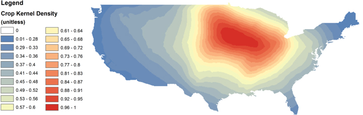
Figure 3. Kernel density index for the crop PFT. This index is generated for each PFT based on the distance and density of surrounding respective PFT land area. The index is used to estimate the geographic location of expansion and contraction of PFT areas that are projected from the integrated assessment model. The index scale represents the lowest density of PFT area (zero) to the highest density of PFT area (one).
Download figure:
Standard image High-resolution image2.1.6. Integration of land classes and climate regimes
Following the spatial distribution of land areas into MODIS PFT land classes, a climate dataset consisting of monthly mean precipitation, temperature, and annual growing degree days (New et al 2002) was spatially superimposed on the land cover data to further disaggregate land classes into temperate, tropical, and boreal climate regions. The climate classes are assigned following the method applied by Bonan et al (2002) and subsequently result in a combination of land classes and climate regimes (table 3) that coincide with those used by the CLM (Oleson et al 2010).
Table 3.
Reclassification of MODIS PFT land classes to CLM PFT land classes
| MODIS PFT numeric code | MODIS PFT (type 5) land class | CLM PFT numeric code | CLM PFT land class |
|---|---|---|---|
| 0 | Water | 1 | Water |
| 1 | Evergreen needleleaf trees | 2 | Needleleaf evergreen tree-temperate (NET temp) |
| 1 | Evergreen needleleaf trees | 3 | Needleleaf evergreen tree-boreal (NETbor) |
| 2 | Evergreen broadleaf trees | 4 | Broadleaf evergreen tree-tropical (BETtrop) |
| 2 | Evergreen broadleaf trees | 5 | Broadleaf evergreen tree-temperate (BETtemp) |
| 3 | Deciduous needleleaf trees | 6 | Needleleaf deciduous tree-all (NDT) |
| 4 | Deciduous broadleaf trees | 7 | Broadleaf deciduous tree-tropical (BDTtropical) |
| 4 | Deciduous broadleaf trees | 8 | Broadleaf deciduous tree-temperate (BDTtemp) |
| 4 | Deciduous broadleaf trees | 9 | Broadleaf deciduous tree-boreal (BDTbor) |
| 5 | Shrub | 10 | Broadleaf evergreen shrub-temperate (BEStemp) |
| 5 | Shrub | 11 | Broadleaf deciduous shrub-temperate (BEStemp) |
| 5 | Shrub | 12 | Broadleaf deciduous shrub-boreal (BESbor) |
| 6 | Grass | 13 | C3 Grass-arctic (C3Garc) |
| 6 | Grass | 14 | C3 Grass-non-arctic (C3G) |
| 6 | Grass | 15 | C4 Grass (C4G) |
| 7 | Cereal crops | 16 | Crops (crop) |
| 9 | Urban and built-up | 17 | Urban (urban) |
| 10 | Snow and ice | 18 | Snow and ice (snow) |
| 11 | Barren or sparse vegetation | 19 | Barren or sparse (sparse) |
| 254 | Unclassified | — | — |
| 255 | Fill value | — | — |
aMODIS land classes were further subdivided by climate regime based on climate rules established by Bonan et al (2002).
2.2. Evaluation
An additional objective of this research was to evaluate whether the downscaling and spatial distribution method used in this research realistically captures recent changes in land cover. Consistency between downscaled land realizations and existing local land cover change trends is one of three downscaling criteria suggested by Van Vuuren et al (2010). The evaluation focuses on agricultural lands in the US since this land class is intensively managed and has the largest annual variation over a short time period (i.e., five years). To independently evaluate the downscaling method and limit the number of confounding variables, a 2010 land realization was generated using MODIS land areas instead of GCAM land areas. Specifically, the 2010 land realization was generated by summing 2010 MODIS PFT land areas per AEZ, thereby generating tabular land areas similar to GCAM output, and then downscaling these data using the 2005 MODIS PFT as the initial baseline land cover data. The difference between the 2010 land realization and 2005 MODIS PFT was then compared to the difference between the actual 2010 MODIS PFT and 2005 MODIS PFT to evaluate whether the downscaling method was capturing the location of land contraction and expansion that actually occurred between years 2005 and 2010. The comparison was conducted by statistically correlating grid cells that changed land classes versus grid cells that did not change. For comparison purposes, the native 2005 and 2010 MODIS land cover data were converted from 500 m to 0.05° resolution.
3. Results and discussion
3.1. Downscaling land cover projections
Land class areas for each AEZ region within the contiguous US were reconciled with MODIS PFT land areas and spatially distributed based on a combination of land class transitions derived from GCAM, a set of land transition priority rules, and kernel density functions for each PFT. This method generates annual gridded data products for 19 land classes that are commensurate with CLM land classes. Twelve of these land classes, representing the majority of land cover in the contiguous US, are illustrated in figure 4.
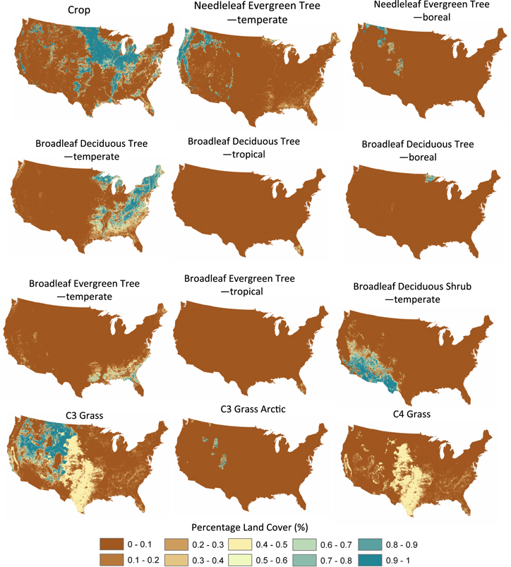
Figure 4. Spatial distribution of GCAM land classes and land areas into CLM PFT land classes based on a combination of GCAM and MODIS land areas per AEZ. This represents baseline conditions in 2005.
Download figure:
Standard image High-resolution imageAs a result of the downscaling process, numerous crop categories were aggregated to one cropland class in the MODIS PFT (figure 4). Conversely, the two forest categories and two woody biomass feedstocks initially combined from GCAM model output were disaggregated to MODIS forest PFTs (figure 4) during the spatial distribution process. The initial reconciling of land areas indicates an excess of MODIS cropland area in AEZ regions 9, 10, and 11 compared to what exists in the baseline GCAM data (table 4). This echoes conclusions by West et al (2010) that cropland area estimated by MODIS PFT land cover is in excess of land area estimated by national inventory data, while MODIS NPP estimates for croplands fall short of those estimated in the inventory data (Li et al 2014). Forest areas increased in the initial reconciling (table 4) with the largest area increase occurring for deciduous broadleaf and evergreen needleleaf, and the largest percentage increase occurring for evergreen broadleaf and deciduous needleleaf. The largest percentage increase in evergreen broadleaf occurred in AEZ 7, and this change represented only 0.15% of the total land area in AEZ 7. No percentage change in any PFT during the initial reconciling exceeded 10% of the total respective AEZ land area.
Table 4.
Total land areas in the MODIS PFT and GCAM land cover data for 2005 and the difference between land areas per AEZ
| AEZ | Evergreen needleleaf | Evergreen broadleaf | Deciduous needleleaf | Deciduous broadleaf | Shrub | Grass | Crop |
|---|---|---|---|---|---|---|---|
| MODIS 2005 (in 103 km2) | |||||||
| 7 | 44 | 0 | 0 | 1 | 703 | 1453 | 141 |
| 8 | 136 | 1 | 1 | 3 | 68 | 509 | 228 |
| 9 | 54 | 4 | 0 | 38 | 28 | 61 | 160 |
| 10 | 74 | 20 | 3 | 380 | 32 | 249 | 646 |
| 11 | 25 | 11 | 1 | 366 | 17 | 202 | 451 |
| 12 | 61 | 170 | 0 | 212 | 71 | 218 | 145 |
| 13 | 38 | 0 | 0 | 1 | 7 | 147 | 10 |
| 14 | 81 | 0 | 1 | 1 | 3 | 55 | 4 |
| 15 | 18 | 0 | 0 | 3 | 0 | 5 | 0 |
| 16 | 3 | 0 | 0 | 0 | 0 | 0 | 0 |
| Total | 534 | 207 | 7 | 1004 | 928 | 2899 | 1784 |
| GCAM2005 downscaled (in 103 km2) | |||||||
| 7 | 72 | 21 | 19 | 10 | 669 | 1338 | 274 |
| 8 | 167 | 4 | 4 | 6 | 49 | 449 | 272 |
| 9 | 57 | 5 | 0 | 40 | 17 | 99 | 124 |
| 10 | 84 | 24 | 5 | 468 | 1 | 298 | 501 |
| 11 | 27 | 12 | 1 | 382 | 0 | 248 | 382 |
| 12 | 81 | 212 | 1 | 288 | 0 | 124 | 162 |
| 13 | 70 | 1 | 2 | 2 | 0 | 104 | 24 |
| 14 | 91 | 0 | 1 | 1 | 0 | 44 | 7 |
| 15 | 21 | 0 | 0 | 3 | 0 | 2 | 0 |
| 16 | 3 | 0 | 0 | 0 | 0 | 0 | 0 |
| Total | 673 | 279 | 33 | 1200 | 737 | 2707 | 1748 |
| GCAM downscaled minus MODIS (in 103 km2) | |||||||
| 7 | 28 | 21 | 19 | 10 | −34 | −115 | 134 |
| 8 | 32 | 3 | 3 | 3 | −18 | −60 | 44 |
| 9 | 3 | 1 | 0 | 2 | −11 | 38 | −36 |
| 10 | 10 | 4 | 2 | 88 | −30 | 50 | −145 |
| 11 | 1 | 1 | 0 | 16 | −17 | 46 | −69 |
| 12 | 20 | 41 | 0 | 75 | −71 | −94 | 17 |
| 13 | 32 | 1 | 1 | 2 | −7 | −43 | 15 |
| 14 | 10 | 0 | 0 | 0 | −3 | −11 | 4 |
| 15 | 3 | 0 | 0 | 0 | 0 | −3 | 0 |
| 16 | 0 | 0 | 0 | 0 | 0 | 0 | 0 |
| Total | 139 | 72 | 26 | 196 | −192 | −192 | −36 |
aUrban, snow, and sparse land classes were included in the analysis, but are shown in this table.
Using the reconciled baseline land distributions (figure 4), future land realizations for each year and for each scenario were generated and archived for public access (West and Le Page 2014). All grass, shrubland, and forest classes were aggregated, respectively, to summarize trends in land cover projections for discussion purposes. Results from 2005 to 2095 in the reference scenario indicate a net replacement of grasslands by croplands (figure 5). In the MP 4.5 scenario, cropland also replaced grassland nationally, with additional replacement of grassland by forests. This is due in part to the economic value placed on terrestrial carbon thereby providing land owners an incentive to afforest and maintain forested land to reduce net CO2 emissions to the atmosphere (Thomson et al 2011, Wise et al 2009). Carbon price policies in GCAM go into effect in 2015 and effects from these policies are seen in the following simulation year (i.e., 2020). The MP 2.6 scenario differs from MP 4.5 with the increase in forest lands occurring earlier in time and with a larger increase in cropland area. The larger increase in cropland area is due in part to increased use of dedicated biomass energy crops (Thomson et al 2013).

Figure 5. Change in PFT land classes from 2005 to 2095 for the (a) reference scenario, (b) mitigation pathway (MP) 4.5, and (c) MP 2.6.
Download figure:
Standard image High-resolution imageDownscaled national land projections reveal regional patterns about the potential impact of socio-economic and environmental factors on land use change decisions. While national trends in land cover change tend to be homogeneously distributed over time in the reference scenario, with a slight increase in croplands driven by increasing food demand, the economic policies implemented in the MPs result in opposite land cover change patterns between the eastern and western US. For example, crop area in the MP 4.5 scenario decreases in the eastern US (i.e., AEZs 10, 11, and 12) while increasing in the western US (i.e., 7, 8, and 9), resulting in a national net increase (table 5). The trend in the MP 2.6 scenario is similar, although the total net area increase in cropland is greater than the MP 4.5 scenario. Downscaling these data indicates that the increase in cropland occurs primarily on the western and southern edge of the Corn Belt and in the western states of Utah and Colorado, replacing mostly grasslands (figure 6). Both the grassland and cropland areas decrease in the eastern US and are replaced by forest land (figure 6). The movement from grassland to croplands, as opposed to a shift from forest to croplands, was also estimated by Hellwinckel et al (2010) using a national agricultural economics model for land cover change projections. Similarly, Sleeter et al (2012) estimated an expansion of agricultural lands to the west and south of the Corn Belt at the expense of grassland to the west and forest to the south in response to A1B and A2 emission scenarios in the US. These spatial patterns highlight the potential influences on land cover from policy-induced changes in the profitability of biofuel crops and forested lands across environmental gradients.
Table 5. Total forest, shrub, grass, and crop area in each AEZ for years 2010, 2050, and 2090.
| AEZ | Forest | Shrub | Grass | Crop | ||||||||
|---|---|---|---|---|---|---|---|---|---|---|---|---|
| 2010 | 2050 | 2090 | 2010 | 2050 | 2090 | 2010 | 2050 | 2090 | 2010 | 2050 | 2090 | |
| Reference scenario (in 103 km2) | ||||||||||||
| 7 | 122 | 122 | 122 | 669 | 650 | 643 | 1338 | 1315 | 1308 | 274 | 316 | 330 |
| 8 | 181 | 178 | 173 | 49 | 45 | 43 | 449 | 424 | 412 | 272 | 304 | 323 |
| 9 | 102 | 100 | 99 | 17 | 16 | 15 | 99 | 92 | 91 | 124 | 134 | 137 |
| 10 | 581 | 563 | 556 | 1 | 1 | 1 | 298 | 277 | 271 | 501 | 540 | 553 |
| 11 | 421 | 411 | 403 | 0 | 0 | 0 | 248 | 232 | 227 | 382 | 407 | 421 |
| 12 | 581 | 578 | 572 | 0 | 0 | 0 | 124 | 119 | 116 | 162 | 171 | 179 |
| 13 | 75 | 76 | 76 | 0 | 0 | 0 | 104 | 103 | 103 | 24 | 24 | 24 |
| 14 | 93 | 93 | 93 | 0 | 0 | 0 | 44 | 44 | 44 | 7 | 7 | 7 |
| 15 | 24 | 25 | 25 | 0 | 0 | 0 | 2 | 2 | 2 | 0 | 0 | 0 |
| 16 | 3 | 3 | 3 | 0 | 0 | 0 | 0 | 0 | 0 | 0 | 0 | 0 |
| Total | 2183 | 2149 | 2122 | 736 | 712 | 702 | 2706 | 2608 | 2574 | 1746 | 1903 | 1974 |
| Mitigation pathway 4.5 scenario (in 103 km2) | ||||||||||||
| 7 | 122 | 158 | 201 | 669 | 604 | 546 | 1338 | 1240 | 1136 | 274 | 401 | 520 |
| 8 | 181 | 263 | 311 | 49 | 32 | 21 | 449 | 324 | 239 | 272 | 333 | 380 |
| 9 | 102 | 127 | 144 | 17 | 10 | 7 | 99 | 65 | 47 | 124 | 140 | 143 |
| 10 | 581 | 692 | 768 | 1 | 1 | 1 | 298 | 191 | 142 | 501 | 498 | 471 |
| 11 | 421 | 528 | 586 | 0 | 0 | 0 | 248 | 163 | 124 | 382 | 360 | 341 |
| 12 | 581 | 637 | 657 | 0 | 0 | 0 | 124 | 78 | 59 | 162 | 152 | 151 |
| 13 | 75 | 87 | 90 | 0 | 0 | 0 | 104 | 98 | 96 | 24 | 19 | 17 |
| 14 | 93 | 99 | 99 | 0 | 0 | 0 | 44 | 43 | 43 | 7 | 2 | 2 |
| 15 | 24 | 25 | 25 | 0 | 0 | 0 | 2 | 1 | 1 | 0 | 0 | 0 |
| 16 | 3 | 4 | 4 | 0 | 0 | 0 | 0 | 0 | 0 | 0 | 0 | 0 |
| Total | 2183 | 2620 | 2885 | 736 | 647 | 575 | 2706 | 2203 | 1887 | 1746 | 1905 | 2025 |
| Mitigation pathway 2.6 scenario (in 103 km2) | ||||||||||||
| 7 | 122 | 190 | 217 | 669 | 569 | 518 | 1338 | 1174 | 1080 | 274 | 471 | 589 |
| 8 | 181 | 313 | 307 | 49 | 25 | 18 | 449 | 268 | 205 | 272 | 346 | 422 |
| 9 | 102 | 142 | 145 | 17 | 8 | 7 | 99 | 52 | 42 | 124 | 140 | 149 |
| 10 | 581 | 762 | 777 | 1 | 1 | 1 | 298 | 156 | 127 | 501 | 463 | 476 |
| 11 | 421 | 585 | 588 | 0 | 0 | 0 | 248 | 135 | 112 | 382 | 330 | 351 |
| 12 | 581 | 660 | 652 | 0 | 0 | 0 | 124 | 64 | 54 | 162 | 143 | 162 |
| 13 | 75 | 90 | 90 | 0 | 0 | 0 | 104 | 96 | 95 | 24 | 17 | 18 |
| 14 | 93 | 99 | 98 | 0 | 0 | 0 | 44 | 43 | 43 | 7 | 2 | 3 |
| 15 | 24 | 25 | 25 | 0 | 0 | 0 | 2 | 1 | 1 | 0 | 0 | 0 |
| 16 | 3 | 4 | 4 | 0 | 0 | 0 | 0 | 0 | 0 | 0 | 0 | 0 |
| Total | 2183 | 2870 | 2903 | 736 | 603 | 544 | 2706 | 1989 | 1759 | 1746 | 1912 | 2170 |
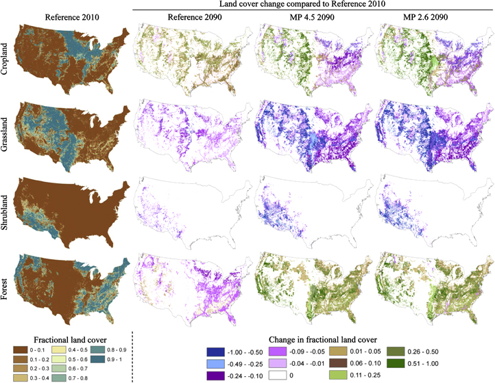
Figure 6. Land cover distribution in 2010 for the reference case and net changes in land cover in 2090 for the reference scenario, mitigation pathway (MP) 4.5, and MP 2.6. Annual gridded projections from 2005 to 2095 are available at http://daac.ornl.gov (West and Le Page 2014).
Download figure:
Standard image High-resolution image3.2. Evaluation
Difference maps of native 500 m resolution MODIS land cover for 2005 and 2010 illustrate a spatially defined area of land cover change around the Corn Belt (figure 7). The Corn Belt is defined as a region of fertile soils, ample rainfall, and intense agricultural production that is centered around Iowa and extends from western Ohio to the eastern portions of North Dakota, South Dakota, and Nebraska. The interior of the Corn Belt experiences little land cover change with respect to movement between croplands and other land cover types. MODIS land cover data indicates that cropland expanded on the western edge of the Corn Belt between 2005 and 2010 and did so at the expense of grasslands (figure 7(b)). This change in land cover is further supported by national inventory data, which estimates a 13 194 km2 increase in corn and soybean land area in the western tri-state region represented by North Dakota, South Dakota, and Nebraska (USDA 2014). The western and southern portions of the Corn Belt are less productive than the interior Corn Belt, thereby less profitable to farm. These lands are biophysically and economically marginal, and are cultivated when prices rise or cropland area is in short supply. Estimates of future land cover change generated from the GCAM model inherently represent these regions of marginality, because changes in land cover and land use are based on cropland production costs including irrigation costs, land rents, average crop yields, and net profits to the farmer.
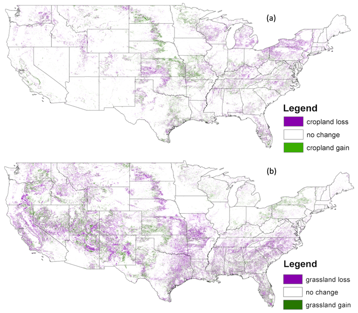
Figure 7. Difference between MODIS PFT Type 5 land cover for 2005 and 2010 at native 500 m resolution with each grid cell representing one PFT. Loss and gain in (a) cropland area and (b) grassland area is relative to the year 2005.
Download figure:
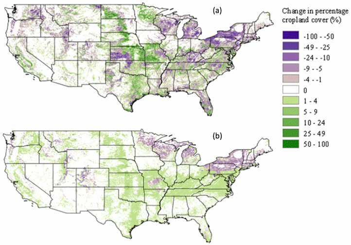
Standard image High-resolution imageTo conduct an evaluation of the downscaling method, we compared the difference between 2010 and 2005 MODIS PFT land cover at 0.05° resolution (figure 8(a)) to the difference between our 2010 downscaled land realization and the 2005 MODIS PFT land cover (figure 8(b)). The comparison is intended to evaluate whether the land cover change is distributed in a manner that matches recent trends in land cover change. In this case, the downscaling procedure captures the geospatial gradient of short-term land cover change on the western and southern edges of the Corn Belt (figure 8(b)). This is particularly important because it illustrates that when our downscaling method is applied to more generalized data at the regional AEZ level (figure 2), the approximation of where land cover change occurs is commensurate with the recent pattern of land cover change in the US.
Figure 8. The difference between (a) 2005 and 2010 MODIS cropland area and (b) 2005 MODIS cropland area and the 2010 land realization, both generated at 0.05° resolution with each grid cell representing fractional coverage for each PFT.
Download figure:
Standard image High-resolution image
There was high correlation between crop PFT land cover in the native 2010 MODIS land cover and the 2010 land realization generated here (r2 = 0.98). Correlations were similar for grass, shrub, and forests with r2 values of 0.86, 0.92, and 0.85, respectively. Correlation between the cropland difference maps (see figure 8), representing only those grid cells that changed, was lower (r2 = 0.83). Correlations between the difference maps for remaining grass, shrub, and forests PFTs were similar with r2 values of 0.72, 0.80, and 0.74. The goal of the evaluation portion of this research was to determine whether the downscaling method provides some level of consistency with existing local scale trends, a downscaling criteria suggested by Van Vuuren et al (2010). The relatively high correlation per grid cell seemingly meets or exceeds this criterion.
The evaluation also reveals two additional observations worth noting. The first observation is the somewhat blocky spatial distribution of cropland expansion along the western edge of the Corn Belt (figure 8(b)). This is due primarily to underlying AEZ boundaries (figure 2). Not coincidently, the expansion and contraction zone of agricultural lands and grasslands lies at the intersection of three narrow AEZ regions (e.g., AEZ 8, 9, and 10) that extend in a North-to-South gradient and are differentiated largely by trends in annual precipitation. The smaller geospatial size of the AEZ boundaries in this area (i.e., AEZ 8 and 9) provide less area with which to reconcile differences in land area statistics and satellite-based land cover, thereby forcing land expansion or contraction into smaller regions. This phenomenon is both less likely and less apparent in larger AEZ regions (e.g., AEZ 7, 11, and 12). The second observation is that the land cover change occurring from 2005 to 2010 is shown in our downscaling method as a net change (figure 8(b)), as opposed to all changes that occurred over the landscape (figure 8(a)). For example, if cropland increases by 100 units and decreases by 50 units in the same AEZ region, our method will capture a net increase of 50 units in the respective region. When using these data for modeling purposes, consideration should be given to whether net versus gross changes in land cover are needed.
Future improvements to this method may include development of a higher resolution (i.e., 0.05°) AEZ grid, as opposed to the existing 0.5° grid, and development of a higher resolution (i.e., 0.05°) kernel density data, as opposed to the current 1.0° data per PFT land cover class. Additionally, data on irrigation versus rainfed land areas, protected lands, and a productivity index that serves as an additional biophysical constraint may also help improve the downscaling and distribution of land cover.
4. Conclusions
Regional data output on land class areas, generated from the GCAM IAM, were reconciled with MODIS land areas and spatially distributed at the 0.05° resolution. This resolution is commensurate with the MODIS land cover product (MCD12C1) for climate modeling. The generation of this product promotes a stronger link between sub-regional and watershed level analyses of carbon, energy, and water cycles with global climate modeling. Results indicate that GCAM predicts changes in land use at the AEZ scale that agree with recent changes in land cover, and this is in large part due to the production costs and net profit data that drive GCAM scenarios. Similarly, the downscaling methodology introduced and evaluated here distributes GCAM land areas to a 0.05° MODIS land cover grid in a manner that captures the recent trends in cropland and grassland expansion and contraction in the US. While it is not possible to forecast the exact percentage change in land classes per grid cell, it is possible to generate land realizations that capture regional trends and do so at a resolution that is useful for sub-regional land management models that are used to assess environmental impacts.
Acknowledgments
This research was conducted under the Pacific Northwest National Laboratory (PNNL) Platform for Regional Integrated Modeling and Analysis (PRIMA) program with Laboratory Directed Research and Development funding. Additional funding used for the integration of land cover statistics and satellite remote sensing was provided by the NASA Earth Sciences Division, North American Carbon Program under Project NNH12AU35I. PNNL is managed for the US Department of Energy by Battelle Memorial Institute.