

Abstract
Seasonal and inter-annual variabilities of biogeochemical variables, including nitrous oxide (N2O), an important climate active gas, were analyzed during monthly observations between 2002 and 2012 at an ocean Time-Series station in the coastal upwelling area off central Chile (36° 30.8'; 73° 15'). Oxygen, N2O, nutrients and chlorophyll-a (Chl-a) showed clear seasonal variability associated with upwelling favorable winds (spring–summer) and also inter-annual variability, which in the case of N2O was clearly observed during the occurrence of N2O hotspots with saturation levels of up to 4849%. These hotspots consistently took place during the upwelling-favorable periods in 2004, 2006, 2008, 2010 and 2011, below the mixed layer (15–50 m depth) in waters with hypoxia and some  accumulation. The N2O hotspots displayed excesses of N2O (ΔN2O) three times higher than the average monthly anomalies (2002–2012). Estimated relationships of ΔN2O versus apparent oxygen utilization (AOU), and ΔN2O versus
  suggest that aerobic ammonium oxidation (AAO) and partial denitrification are the processes responsible for high N2O accumulation in subsurface water. Chl-a levels were reasonably correlated with the presence of the N2O hotspots, suggesting that microbial activities fuelled by high availability of organic matters lead to high N2O production. As a result, this causes a substantial N2O efflux into the atmosphere of up to 260 μmol m−2 d−1. The N2O hotspots are transient events or hot moments, which may occur more frequently than they are observed. If so, this upwelling area is producing and emitting greater than expected amounts of N2O and is therefore an important N2O source that should be considered in the global atmospheric N2O balance.
Export citation and abstract BibTeX RIS

Content from this work may be used under the terms of the Creative Commons Attribution 3.0 licence. Any further distribution of this work must maintain attribution to the author(s) and the title of the work, journal citation and DOI.
1. Introduction
Nitrous oxide is a major climate modifying gas (Crutzen 1970) whose production depends on the concentration of O2, organic matter (OM) and bioavailable N compounds such as  and
and  (Codispoti et al 2001). Globally, oceans are thought to add around 4 million tons of N2O to the atmosphere each year, but like other greenhouse gases, much of the N2O exchanged with the atmosphere comes from coastal regions such as upwelling systems (Nevison et al 1995, 2004). There, highly supersaturated N2O conditions in the surface waters mainly arise from the upwelled subsurface waters, where N2O production is accelerated by microbial activities occurring in sinking particles hosted in hypoxic waters (Codispoti et al 2001, Bange 2008).
The properties (variables) of the ocean are changing taking into account acidification, increasing temperatures and deoxygenation, among other factors (Sarmiento et al 2004, Doney et al 2009, Keeling et al 2010), which may influence oceanic N2O inventories (Bange et al 2010). Some studies have showed that O2 minimum zones (OMZ) in the oceans are expected to expand as the world warms (Stramma et al 2008, Keeling et al 2010) affecting N2O production. N2O, on the other hand, is mainly formed as a byproduct during nitrification, including the aerobic oxidation of  to
to  (AAO) and nitrifier denitrification (i.e.
  to N2O) (Poth and Focht 1985), nitrate-ammonification, the fermentative conversion of
  to
to  and partial denitrification, the anaerobic and dissimilatory reduction of
  /
/ to N2O (Codispoti and Christensen 1985, Bange 2008). As O2 decreases to less than 20 μmol L−1, N2O production by AAO, associated with both archaea and bacteria (Santoro et al 2011, Löscher et al 2012), is intensely increased (Goreau et al 1980). However, if O2 becomes exhausted and falls below suboxia, total denitrification takes place, a process by which N2O can be dissimilatively reduced to N2 (Codispoti and Christensen 1985). However, it is very difficult to determine whether these pathways operate individually or interact as coupled mechanisms.
Wind stress is the main physical factor regulating surface gas distribution and its outgassing (Wanninkhof 1992). This is particularly relevant in the coastal upwelling region; thus intensification/reduction of upwelling-favorable winds, a phenomenon that may be associated with global warming (Bakun 1990), could potentially affect microbial activities involved in N2O cycling, and therefore, its temporal dynamics (Capone and Hutchins 2013). This effect is due to the role of wind in ocean ventilation and also in supplying nutrients to surface waters, which have a concomitant effect on primary production (Chl-a and nutrients) and O2 consumption (Gruber 2011).
Shipboard time-series provide new insights into spatial–temporal variability underlying ecosystem change and act as a key tool in forming our knowledge about connectivity between changes in ocean climate and biogeochemistry (Church et al 2013, Taylor et al 2012). Regarding coastal observations, a small number of examples exist, such as the western Indian Ocean continental shelf and some estuarine systems (Naqvi et al 2010). In this study, we have examined the seasonal cycle and the inter-annual variability of N2O along with other biogeochemical variables from the Center for Oceanographic Research in the South Pacific (COPAS) time series obtained from August 2002 to August 2012 to gain a better insight into N2O variability in coastal waters and its associated exchange with the atmosphere.
2. Material and methods
2.1. Sample locations
A fixed station, known as Station 18 (St. 18) at the COPAS center, was sampled regularly at approximately 30 day intervals from July 2002 to August 2012 (figure 1). St. 18 is located over the continental shelf off central Chile at 10 nm (∼18 km) from the shoreline (36°30.80'S; 73°7.75'W) and 92 m depth (http://copas.udec.cl/). Continuous profiles of temperature, salinity, O2, fluorescence, and photosynthetically active radiation (PAR) were obtained using a CTD to measure conductivity, temperature and depth (CTD model SBE-25). Seawater was sampled using a 10 L Niskin bottle mounted on a 10 bottle rosette. Samples for gases (O2, N2O), nutrients and pigments (in this correlative temporal order) were obtained at nine depths distributed between the surface and 92 m depth (2/5, 10, 15, 20, 30, 40, 50, 65 and 80 m depth). Triplicate samples were taken for O2 (in iodimetric bottles immediately fixed) and for N2O (in 20 mL gas chromatography (GC) vials). Preservation was carried out through the addition of 50 μL of saturated mercuric chloride (Tilbrook and Karl 1995) and the GC vials were immediately sealed with a butyl-rubber septum and aluminum cap avoiding air bubbles and, then stored in darkness until analysis. From each sample depth syringes were connected directly to the spigot of the Niskin bottles to obtain triplicate nutrient samples (

 and Si(OH)4), filtered through a 0.45 μm Uptidisc adapted to the syringe, and then stored at −20 °C, whereas for Chl-a, 100 mL of seawater was filtered (triplicate) onto a glass-fiber filter (GF/F) and the filter was immediately frozen.

Figure 1. Study area showing the continental shelf bathymetry off central Chile and the location of St. 18 (36°30.80'S-73°07.75'W).
Download figure:
Standard image High-resolution image2.2. Chemical analysis
O2 was analyzed by the Winkler method using an automatic measurement system. For N2O analysis, within each GC vial, a headspace was created adding 5 mL of ultrapure helium (He) using a 5 mL gas-tight syringe and N2O dissolved in the seawater was measured through gas–liquid equilibration in the vial at 40 °C for 15 min under agitation (using a headspace autosampler device, HP Agilent), followed by quantification via GC. N2O was analyzed in a Varian 3380 GC with an electron capture detector (ECD) at 350 °C, and using a capillary column and injector operated at 60 °C and 250 °C, respectively, and connected to the mentioned autosampler (Farías et al 2009). Five-point calibration curves were constructed using He and 0.1, 0.5, 1 and 100 ppm N2O standards (Mathison gas mixture). Additionally, for the calibration curve, prepared compressed dry air was used with a 0.320 mole dry fraction of N2O from NOAA (http://www.esrl.noaa.gov/gmd/ccl/). The ECD detector lineally responded to this concentration range, which was equivalent to a range of dissolved N2O in seawater of about 7–1500 nmol L−1 (T ∼ 18 °C and S ∼ 35). The analytical error for the N2O measurements was about 3%. The uncertainty of the measurements was calculated from the standard deviation of the triplicate measurements by depth. Samples with a variation coefficient higher than 10% were not taken into account for the N2O database. Nutrients were analyzed by standard manual (from 2002 to 2009) or automated (from 2009 to 2012, autoanalyzer SEAL Analytical) colorimetric methods (Grasshoff et al 1983). Chl-a was analyzed by fluorometry (Turner Design AU-10) according to standard procedures (Parsons et al 1984).
2.3. Data analysis
In order to interpret the vertical and temporal variation of N2O, the water column was divided as follows into two layers according to density and O2 gradient (more details in Farías et al 2009): 1) the mixed and illuminated layer delimited by the base of the mixed layer (ML); 2) the subsurface waters from the base of the ML to the water overlying the sediments (90 m depth). This layer included the oxycline (a layer where O2 levels widely fluctuated but always remained higher than 4.4 μmol L−1) and bottom water (a layer where levels of O2 were as low as 4.4 μmol L−1, generally from 65 to 90 m depth).
N2O solubility was estimated according to Weiss and Price (1980) based on in situ temperature and salinity. Delta or excess of N2O, a measure to diagnose the apparent production of N2O in different water masses (Nevison et al 1995, 2003) was calculated as ΔN2O = [N2O]in situ − [N2O]eq, where [N2O]in situ is the measured concentration of N2O, and [N2O]eq is the concentration of N2O in equilibrium with the atmosphere at the time of the last atmospheric contact. Atmospheric values, at the time in which samples were taken, came from the NOAA/ESRL program register of N2O hemispheric and global monthly means (http://www.esrl.noaa.gov/gmd/hats/combined/N2O.html).
Monthly anomalies of environmental variables, for example N2O, were estimated as
where, xN2O is the discrete value at a certain depth and time, and  is the average value for the whole 2002–2012 period, and σN2O is the respective standard deviation of the dataset.
N2O hotspots were defined as exhibiting a ΔN2O three times higher than the average monthly ΔN2O anomaly at each depth range, i.e.

where, ΔN2O is the monthly estimated N2O anomaly, and  is the average N2O anomaly for the entire water column.
N2O flux through the air–sea interface was determined using the following equation, modified by Wanninkhof (1992):
where, kw is the transfer velocity from the surface water to the atmosphere, as a function of wind speed, temperature and salinity from the ML, Cw is the mean N2O concentration in the ML and Ceq is the gas concentration in the ML expected to be in equilibrium with the atmosphere, according to Weis and Price (1980). The ML depth was calculated using a potential density-based criterion of Kara et al (2003).
Gas transfer velocity was calculated according to Wanninkhof (1992) or W92, estimated to be the best parametrization for the study area. Wind speed and direction based on a six hourly register were obtained from a permanent meteorological station located at Carriel Sur (http://www.meteochile.gob.cl/) that is considered to be a coastal station and meets with international standards. These data were compared with those obtained from satellite observations of ocean winds based on QuikSCAT (2002–2009) and ASCAT (2010–2012).
Cumulative alongshore (south–north) wind stress was obtained using a running mean (10-day) wind stress calculated to eliminate the intra- and inter-daily variability (Barth et al 2007). Wind stress was calculated according to Nelson (1977):
where Cd is the drag coefficient of wind at 10 m above sea level and corresponds to the value of 0.0013 (Kraus 1972), ρair is the air density and corresponds to the value 1.22 kg m−3.  is the wind speed in m s−1 and ν is the meridional component of the wind speed in m s−1.
N2O, O2, 
 and Chl-a inventories were calculated through numerical integration of data at 1 m increments (linear interpolation) based on at least 4–6 sampled depths per layer. Spearman correlations (Rho) were determined for N2O, Chl-a, and nutrient inventories estimated in the surface and subsurface layers. The threshold value for statistical significance was set at p < 0.05. Multiple comparison procedures for all pairwise comparisons among seasonal means were made with a t-student test, with a previous application of the Shapiro–Wilk test to check a normally distributed population. The threshold value for statistical significance was set at p < 0.05.
3. Results
3.1. N2O content in the water column
Time series vertical distributions of O2, Chl-a,  and N2O are shown in figure 2. Chl-a in surface waters fluctuated between 0.1 and 53.15 μg L−1 (mean ± SD = 3.63 ± 5.65) and revealed a marked seasonal cycle with maximum values in spring–summer (upwelling period) and minimum values (<1.00 μg L−1) in wintertime (non-upwelling period) (figure 2(a)). Temporal variability of O2 stands out as the predominant seasonal signal of all oceanographic variables (figure 2(b)). Each year, a winter oxygenation throughout the water column is followed by a gradual deoxygenation (undersaturated levels) in the oxycline and the bottom layers, commencing in September/October and lasting until April. Each spring–summer, the oxycline and the bottom waters showed a decrease in the O2 content reaching values as low as 1 μmol L−1, creating a suboxic/anoxic environment in the bottom waters (close to the sediments), and also a marked oxycline in depths as shallow as 20 m (figure 2(b)).

Figure 2. Temporal variability of parameters in the water column: (a) chlorophyll-a (μg L−1); (b) dissolved oxygen (μmol L−1); (c) nitrite (μmol L−1); and d) nitrous oxide (nnol L−1) throughout the study period (August 2002–2012). Samples from St. 18 located over the continental shelf off central Chile. Note that the scale of N2O concentration was limited 200 nmol L−1 and extremely high values were removed in order to smooth the inter-annual variability.
Download figure:
Standard image High-resolution image
 which is a nutrient with a specific sensitivity to O2 levels, showed highly variable concentrations, ranging from 0 to 11.7 μmol L−1 (mean ± SD = 0.56 ± 0.99) (figure 2(c)). Extremely low values were detected in the surface layer, and some middle values up to 2.5 μmol L−1 at the oxycline (figure 2(c)); whereas during the summer higher values (up to 11.7 μmol L−1) were observed in the bottom layer (associated with suboxic waters). N2O varied from 2.92 nmol L−1 or 28.3% saturation (bottom water, 90 m depth) to 492 nmol L−1 or 4849% saturation, having a mean ± SD of 39.4 ± 29.2 nmol L−1 in the oxyclines (20–64 m depth) and a mean ± SD of 37.6 ± 23.3 nmol L−1 in the bottom waters (65–90 m depth) (figure 2(d)). During mid-autumn and winter, N2O levels were relatively low with occasional undersaturation in the surface layer. Conversely, in spring–summer a large accumulation of N2O was observed as O2 decreased at the oxyclines and the bottom layers (figure 2(d)); however in late summer and early autumn N2O levels as low as 30% saturation were observed in the bottom waters close to the sediments, coinciding with an extremely low O2 concentration (anoxia), and indicating that N2O is being consumed in this layer.
Besides the seasonal cycles described for these variables, an inter-annual variability is also evident, particularly for N2O. Monthly anomalies for Chl-a, O2,  and N2O are illustrated in figure 3. Inter-annual variability was clearly visible during the occurrence of N2O hotspots (figure 2(d)), with very high saturation during December 2004 (up to 2442%), January 2006 (up to 1583%), January 2008 (up to 2097%), December 2008 (up to 2066%), January 2010 (up to 1574%) and November 2011 (up to 4849%). In addition, N2O excess (ΔN2O), the difference between observed N2O and the expected N2O concentration at equilibrium with the atmosphere, was analyzed to eliminate the majority of N2O variability caused by changes in seawater temperature and salinity (figure 4(a)). The monthly anomalies of ΔN2O highlighted the presence of N2O hotspots which contained at least ΔN2O three times higher than the average monthly ΔN2O (figure 4(b)).

Figure 3. Temporal variability of anomalies in the water column of (a) chlorophyll-(a); (b) dissolved oxygen; (c) nitrite; and (d) nitrous oxide during the study period (August 2002–2012) at the St. 18.
Download figure:
Standard image High-resolution image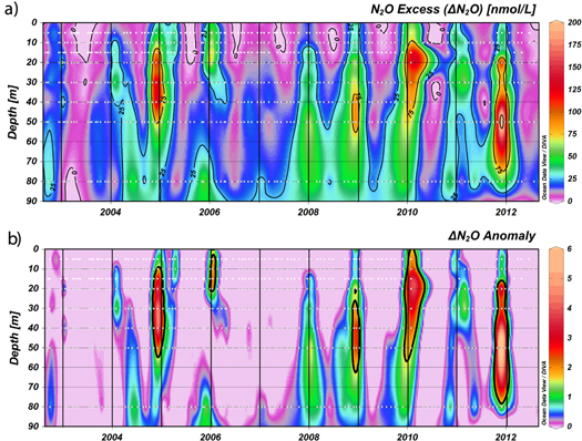
Figure 4. Temporal variability in the water column of (a) N2O excess (nmol L−1); and (b) the anomaly of N2O excess during the study period (August 2002–2012) at the St. 18.
Download figure:
Standard image High-resolution imageOceanographic/biogeochemical profiles obtained during the presence of hotspots are shown in figure 5. In general, the N2O hotspots developed at the oxycline layer, below the ML until 50 m depth and under variable O2 conditions but always in a range of hypoxic conditions (higher than 4.4 μmol L−1, except in November 2011) and with some  accumulation (from 0.53 to 2.53 μmol L−1). Furthermore, the N2O hotspots were always immersed in a layer with high
  and
and  content, ranging from 7.94 to 35.2 and from 1.03 to 2.32 μmol L−1, respectively.
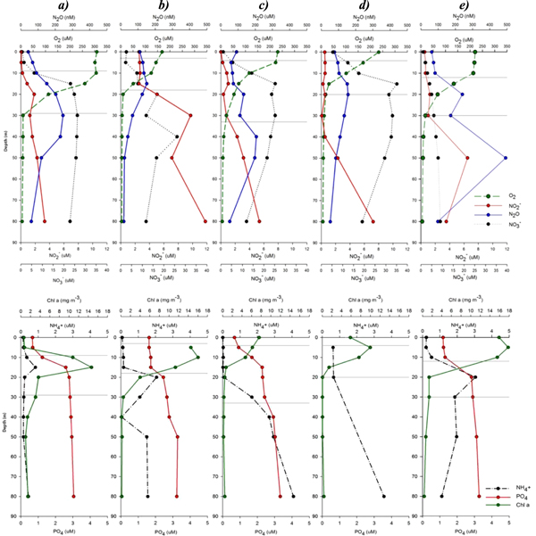
Figure 5. Vertical profiles of oceanographic variables during the N2O hotspot presence. Arrows indicate the location of N2O hotspot core depth during the years (a) 2004; (b) 2006; (c) 2008; (d) 2010; and (e) 2011.
Download figure:
Standard image High-resolution imageTable 1 presents the annual mean inventories of N2O, O2, Chl-a, and  estimated in the surface and subsurface layer from September to March during the sample period. Cumulated surface wind stress for the whole upwelling period is also included. Significant differences were found among mean inventories for all environmental variables estimated for the yearly spring–summer period (p < 0.05) and indicated differences between upwelling seasons. Additionally, table 1 shows that the majority of N2O was accumulated in the oxyclines, which on average accounts for 72% of the total N2O inventory in the water column over the study period, contrasting with 21% of the total inventory that accumulates in the bottom layer.
Table 1. Monthly averages of from nitrous oxide inventories. Chlorophyll-a, nitrate and nitrite estimated during the upwelling season (spring–summer) in both the mixed and subsurface layers, and the cumulated wind stress over the same period from the COPAS time-series station.
| Sept–March | Nitrous Oxide nmol m−2 | Chlorophyll-a mg m−2 (c) | Nitrate μmol m−2 | Nitrite μmol m−2 | Wind Stress N m−2 210 days | |
|---|---|---|---|---|---|---|
| 2002–2003 | ML | 1036 ± 81 | 455 ± 55 | 205 ± 33 | 25 ± 4 | 1459 ± 15 |
| SSL | 7293 ± 471 | 5881 ± 101 | 233 ± 23 | |||
| 2003–2004 | ML | 1068 ± 117 | 280 ± 66 | 706 ± 112 | 13 ± 2 | 2253 ± 9 |
| SSL | 10440 ± 546 | 8280 ± 152 | 212 ± 52 | |||
| 2004–2005a | ML | 2877 ± 417 | 454 ± 89 | 1060 ± 135 | 41 ± 5 | 2376 ± 11 |
| SSL | 23 414 ± 2738 | 10 492 ± 349 | 287 ± 30 | |||
| 2005–2006a | ML | 1203 ± 131 | 245 ± 38 | 160 ± 37 | 21 ± 5 | 3576 ± 9 |
| SSL | 13 171 ± 1089 | 7726 ± 194 | 596 ± 121 | |||
| 2006–2007 | ML | 671 ± 44 | 152 ± 18 | 504 ± 62 | 15 ± 1 | 2446 ± 9 |
| SSL | 9642 ± 252 | 10 824 ± 324 | 195 ± 24 | |||
| 2007–2008 | ML | 866 ± 67 | 236 ± 36 | 680 ± 62 | 15 ± 2 | 2457 ± 9 |
| SSL | 10 084 ± 528 | 8176 ± 349 | 78 ± 6 | |||
| 2008–2009a | ML | 2317 ± 135 | 561 ± 81 | 1306 ± 147 | 30 ± 4 | 4096 ± 17 |
| SSL | 20 502 ± 2599 | 8778 ± 129 | 171 ± 41 | |||
| 2009–2010a | ML | 1076 ± 159 | 44 ± 3 | 598 ± 308 | 14 ± 5 | 4013 ± 15 |
| SSL | 10 928 ± 3026 | 3834 ± 417 | 102 ± 42 | |||
| 2010–2011 | ML | 1950 ± 242 | 293 ± 66 | 849 ± 139 | 30 ± 6 | 3802 ± 11 |
| SSL | 15 365 ± 1323 | 7378 ± 282 | 253 ± 33 | |||
| 2011–2012a | ML | 2137 ± 229 | 384 ± 40 | 1182 ± 148 | 30 ± 4 | 1164 ± 3 |
| SSL | 29 795 ± 4912 | 12 589 ± 306 | 328 ± 56 |
aDenotes upwelling periods during N2O hotspot presence; bMixed layer (ML) and subsurface layer (SSL); cInventories estimated in surface (the mixed layer) and subsurface waters (the latter included the oxycline and the bottom layer).
3.2. Air–sea N2O exchange and relationships among environmental variables
The wind speed and alongshore wind speed ranged from 0.51 to 26.46 m s−1 (figure 6(a)) and −15.47 to 9.36 m s−1, respectively. The meridian component of the wind, which provoked favorable upwelling events, was observed more frequently in spring–summer and it occurred in total for approximately 61.26% of the whole year. The cumulated wind stress (10-day running mean) varied from −1.43 to 0.68 N m−2 10 days and clearly showed that the cumulative upwelling-favorable wind stress occurred during the spring–summer time (figure 6(b)). Sea surface temperature (SST in °C), measured at 10 m depth to avoid the effect of solar radiation, presented a similar pattern to the cumulated wind stress, indicating that cold subsurface water is being upwelled to the surface layer (figure 6(c)). N2O fluxes varied between −10.47 and 260.2 μmol m−2 d−1 (mean ± SD = 27.88 ± 44.5) (figure 6(d)). Temporal trends in N2O fluxes also showed a marked seasonal pattern, being lower (influx) during the non-favorable upwelling periods and higher (efflux) during the favorable upwelling periods; this coincided with supersaturated N2O conditions in the ML, with levels ranging from 71.85 to 1428% saturation over the whole study period. The highest N2O fluxes coincided with the presence of the N2O hotspots (figure 6(d)).

Figure 6. Time series of (a) wind speed (m s−1); (b) along shore wind stress on surface (N m−2 days); (c) sea surface temperature (SST) measured at 10 m depth (°C); and (d) estimated air–sea N2O fluxes (μmol m−2 d−1), at St. 18. Vertical green lines indicate the dates at which the N2O hotspots were present.
Download figure:
Standard image High-resolution imageTable 2 shows Spearman correlations carried out among several environmental variables as cumulative wind stress, SST, Chl-a and inventories of N2O,  and
and  in the surface and subsurface layer. Cumulative wind stress correlated negatively with SST, whereas it correlated positively with Chl-a and N2O inventories, but no correlations were found between wind stress and nutrient inventories (table 2). These correlations imply that more intensive upwelling favorable winds provoke a rise of cold and nutrient- and gas-rich subsurface water to the surface, fertilizing and allowing the accumulation of phytoplankton biomass in the surface water and accelerating the gas exchange across the air–sea interface (figure 6(d)). However, these nutrients were more rapidly consumed and assimilated by phytoplankton than the rates at which they were supplied at the surface by upwelling events. In addition, N2O inventories in surface and subsurface layers correlated reasonably well with Chl-a inventories in the surface layer (table 2). Since the N2O hotspots were only present during upwelling-favorable winds, this pattern would suggest that these structures were controlled by the wind. However, no significant correlation was found between the N2O inventory at surface layer and SST, suggesting that the dynamics of N2O was not just controlled by physical processes (table 2). By contrast, the content of N2O in surface and subsurface layer was related positively to Chl-a level and the NO2- inventory at surface waters.
Table 2. Spearman correlation coefficients among cumulative wind stress, N2O inventories and several biogeochemical variables in the COPAS time series station.
| Cumulative Wind Stress (Nm−2 10 days) | sur N2O (μmol m−2) | sub N2O (μmol m−2) | ||||
|---|---|---|---|---|---|---|
| Rho | p | Rho | p | Rho | p | |
| SSTa | −0.40 | 0.00 | −0.07 | 0.45 | −0.20 | 0.04 |
| Chl-ab | 0.51 | 0.00 | 0.47 | 0.00 | 0.24 | 0.01 |
| sur N2Ob | 0.43 | 0.00 | — | — | — | — |
| sub N2Ob | 0.24 | 0.01 | — | — | — | — |
sur  b
b
|
0.00 | 0.97 | 0.32 | 0.00 | −0.33 | 0.00 |
sub  b
b
|
−0.03 | 0.76 | −0.03 | 0.77 | 0.12 | 0.20 |
sur  b
b
|
0.00 | 0.92 | 0.39 | 0.00 | −0.43 | 0.00 |
sub  b
b
|
0.17 | 0.06 | −0.17 | 0.06 | 0.23 | 0.10 |
aSST in °C. bBiogeochemical variables are estimated as inventories in surface (sur) and subsurface (sub) layer.
4. Discussion
The continental shelf off central Chile is subject to SW wind stress (figure 6(b)) that produces upwelling events during the austral spring–summer and affects most of the physical variables, such as temperature and salinity (Sobarzo et al 2007). The fertilization of the photic zone is the most notable consequence of this process, which can sustain high phytoplanktonic development, primary production, and the subsequent intense respiration of produced OM (figure 2) (Daneri et al 2012, Farías et al 2009). Thus, the phytoplankton standing stock increased throughout the upwelling season, as illustrated by the progressive accumulation of Chl-a in the surface water (figure 2(a)), with a subsequent buildup in the particulate OM occurring at the oxycline and the bottom layers (Farías et al 2009). This leads to an intense aerobic respiration of sinking organic particles, which along with the presence of the eastern Southern Pacific's OMZ causes a decrease in O2 to anoxic levels (Ulloa et al 2012). This stimulates dissimilative processes involved in N cycling, particularly those associated with N2O production, such as nitrification and denitrification (Codispoti and Christensen 1985).
Some coastal upwelling areas show a rapid seasonal transition from oxic to anoxic conditions. In the study area, this phenomenon was observed throughout the vertical O2 distribution (figure 2(b)), where conditions transitioned from relatively homogenous and oxygenated to a very shallow and sharp oxycline; as a result this influences the N2O distribution (Cornejo et al 2007). This transition is accompanied by N2O accumulation at the oxyclines (December–January) and consumption within the bottom layers (March–April) (figure 2(d)). Marked N2O accumulation has previously been observed in only a few coastal time-series sites associated with the continental shelf and coastal upwelling, such as those off central Chile and West India, (Naqvi et al 2010). Such N2O accumulations (up to several hundred nM) were related with low O2 levels, where significant amounts of N2O can temporarily accumulate during the short transition time, while the system is changing its oxygen regime (Bange et al 2010, Bakker et al 2014).
N2O hotspots are defined as patches that show disproportionately high reaction rates relative to the surrounding water according to McClain et al (2003). In our study area (off central Chile), they have ΔN2O three times higher than the average monthly ΔN2O (figure 4). These hotspots were present between November and January at the oxyclines (15–50 m range depth) with hypoxic rather than suboxic levels (higher than 4.4 μmol L−1) and with some  accumulation, which seems to form the primary
  maxima (figure 5). This contrasts with
  accumulation observed in the bottom water under suboxic/anoxic conditions (figure 2(b)) whose origin seems to be related to dissimilative
  reduction (Lomas and Lipschultz 2006). This situation was dissimilar to that reported by Naqvi et al (2000) in the western Indian continental shelf; they found strong N2O accumulation and the occurrence of sulphide in open coastal waters. However, in this case, the increased N2O production seemed to be caused by the addition of anthropogenic
  associated with strong river runoff and a subsequent reduction to N2O (i.e., partial denitrification).
According to the observed correlations, upwelling-favorable wind stress modulated the seasonal N2O content in surface and subsurface waters (table 1). However the N2O hotspots were not necessary associated with the strongest wind stress (figure 6(b)), nor with the colder waters (SST) upwelling/rising from the subsurface (figure 6(c)). The presence of the N2O hotspots was well correlated with Chl-a (table 2), revealing the significance of the phytoplanktonic biomass in providing OM and the concomitant mineralization products ( and N2O).
4.1. Origin of N2O accumulated in the hotspot
Based on the O2/N2O emission ratio observed in atmospheric records (Lueker et al 2003), marine N2O is predominately being sourced from nitrification. Considering correlations between ΔN2O versus AOU and ΔN2O versus  it is possible to determine if N2O production is related to O2 consumption and
  production, due to OM remineralization coupled with nitrification (Yoshinari 1976, Nevison et al 2003). Figure 7 illustrates the relationship among these parameters and variables with all data (figures 7(a), (b)) a significant correlation of ΔN2O versus AOU and ΔN2O versus
  (respectively Rho = 0.40, p < 0.05 and Rho = 0.34 p < 0.05) is observed; similar results were obtained with data from the upper oxycline (i.e., 20 m depth, respectively, Rho = 0.53 p < 0.05 and Rho = 0.43p < 0.05; figures 7(c), (d)), indicating that N2O and
  are being produced in parallel to O2 consumption by nitrification. However, correlations between these parameters lose statistical significance as the estimates are carried out with data from the deepest layers (i.e., 50 and 80 m depth). In fact, a
  consumption was observed at O2 levels as low as ∼5 μmol L−1, which implies that an advected/diffused denitrification signal from the bottom layer or sediment, and/or an in situ denitrification at the oxyclines is/are occurring simultaneously with the nitrification. Indeed, when these relationships (ΔN2O versus AOU and ΔN2O versus
  were estimated from 50 m (respectively Rho = 0.20 p < 0.05 and 0.30 p < 0.05; figures 7(e), (f)) and 80 m depth (respectively, Rho = 0.10 p = 0.36 and Rho = 0.23 p < 0.05; figures 7(g), (h)), they revealed a strong denitrification observable by an intense
  and N2O consumption.

Figure 7. Relationship found between ΔN2O (nmol L−1) versus AOU (μmol L−1), and ΔN2O versus  (μmol L−1) in the water column with, respectively, (a), (b) the whole data set taken from 2002 to 2012; (c), (d) the data from 20 m depth; (e), (f) data from 50 m depth; and (g), (h) data from 80 m depth. Each graph includes a linear regression model between both parameters and the black line indicates a linear regression line.
Download figure:
Standard image High-resolution image
Regarding the processes responsible for the observed N2O distribution in the study area, high AAO rates at the oxyclines were observed in association with high  regeneration rates (Fernandez and Farías 2012), however at the oxyclines and possibly also at the bottom waters, AAO appeared to be coupled to
  and
and  reduction to N2O (partial denitrification), which has been previously reported in the study area (Fernandez and Farías 2012, Galán et al 2014). With respect to the microbes involved in these processes, beside AAO bacteria, AAO archaea also play an important role as ammonia oxidizers at oxyclines in the central Chilean upwelling (Molina et al 2010). Some archaea have a high affinity for
  (Martens-Habbena et al 2009), efficiently producing N2O as a by-product (Santoro et al 2011); sulfur-oxidizing γ-proteobacteria are abundant and dominant at the oxyclines in our study area, and additionally, they have the ability to reduce dissimilative
  and
and  and carry out a process known as chemolithoautotrophic denitrification (Murillo et al 2014), which could be producing N2O throughout partial denitrification (Galán et al 2014).
4.2. N2O exchange across air–sea interface
Another observed consequence of the upwelling processes was a strong outgassing. In fact, the contribution from coastal upwelling has been estimated as 0.2 ± 0.14 Tg N2O-N yr–1, which represents ∼5% of the total ocean source (Nevison et al 2004), despite representing less than 1% of the total surface of the ocean. Most of these coastal upwellings, which encompass eastern boundary systems, have been recognized as significant N2O emission areas, such as those associated with the Arabian Sea (De Wilde and Helder 1997, Naqvi et al 2005), the eastern South Pacific (Cornejo et al 2007, Charpentier et al 2010) and west Africa, including the Benguela current and Mauritanian upwelling (Wittke et al 2010, Kock et al 2012).
Given the proximity of the N2O hotspots to surface water (figure 5), they could be shifted closer to the surface by the piston effect of the SW wind. Indeed, air–sea N2O fluxes vary in magnitude throughout the year, changing from negative to positive values (figure 6(d)); however, for the majority of the year there is a strong efflux of N2O, indicating that the area behaves as a strong gas source towards the atmosphere. It is important to note that fluxes were estimated with wind data that came from a continental location (close to the coast); this may indicate the occurrence of a retarding or frictional force on the wind that could reduce the wind strength magnitude. In fact, comparison of these data with those obtained from satellites indicates that these data underestimate the N2O air–sea exchange by about 20%. Taking into consideration that wind is highly variable with bursts of intensity (up to 26 m s−1), the parametrization of W-92 should be the most appropriate for the study area.
During the presence of hotspot structures, N2O effluxes were up to one order of magnitude higher than the average flux estimated during the entire decade (figure 6(d)), and almost two orders of magnitude higher than the global ocean estimate of about 3 μmol m−2 d−1 (Nevison et al 1995). Breaking down the variation of N2O flux across the air–sea interface into decadal, seasonal, and inter-annual variation facilitates a more precise temporal scaling to assess the impact of the gas exchange on the atmosphere. If we consider that the observed dynamic is occurring on Chile's continental shelf (41 105 km2), this coastal area contributes, based on a weighted average (upwelling and non-upwelling representative of 60% and 40% of the year, respectively), 20.7 Gg N2O-N per year, which is a significant N2O contribution/source that should be considered in the global balance of atmospheric N2O. Furthermore, if we take into consideration that the N2O hotspots may occur more frequently than observed during this study's sampling cycle (at intervals of 30 days or more), this contribution appears to be further underestimated. In fact, when the N2O efflux data was removed for periods during the N2O hotspots' presence, the annually weighted average was reduced to 13.5 Gg N2O-N; therefore, the importance of the area as a source of N2O could be scaled up. As a result transient events rather than long-term steady-state conditions have been proposed to govern N2O production in coastal areas subjected to eutrophication and hypoxia (Naqvi et al 2000).
There exists the possibility that N2O dynamics act as hot moments, which are defined as short periods of time exhibiting disproportionately high reaction rates relative to longer intervening time periods (McClain et al 2003). In this sense, high frequency events (at the weekly and intra-seasonal scales) could be affecting the presence of hot moments. In general, upwelling-favorable winds work with quasi-weekly upwelling pulses, consisting of an alternation in the winds and/or change in wind intensity; with respect to the southern hemisphere, this may vary from southerly and intense (active upwelling) to northern and decreased winds (upwelling relaxation) (Send et al 1987, Rutllant and Montecino 2002). Over a 5- to 10-day time scale this active-relaxing cycle affects both microbial communities and the accumulation of biomass, and primary production rates and microbial community composition (Rutllant and Montecino 2002, Wilkerson et al 2006, Du and Peterson 2009). For example, for effective Chl-a accumulation an optimal window of 3–7 days of relaxed winds was required following an upwelling pulse. Thus, N2O hot moments may occur during the relaxing phase of the upwelling process, and therefore would require a weekly and intra-seasonal study scale in order to resolve the frequency of these events.
Within the study region there are no clear decadal trends of an increase in phytoplanktonic biomass or an intensification of hypoxic conditions in subsurface waters regarding the analysis of the COPAS time series; however, phenomena such as the cooling of surface waters and intensification of coastal wind patterns have been reposted by Falvey and Garreaud (2009) in the study area. Therefore, we recommend further study on the physical forcing (i.e. ENSO and even global warming) mechanisms that may be affecting biogeochemical processes involved on N2O production and exchange across the air–sea interface.
Acknowledgments
Both the crew of R/V Kay Kay (II) and the Dichato Marine Station of the University of Concepción provided valuable help during fieldwork, as well as all participating colleagues in the COPAS time series (COPAS program), who provided the core measurements, particularly Carmen Morales and Valeria Anabalon who carefully checked the Chl-a data. We also appreciate the work done since the beginning of COPAS TS by Mauricio Gallegos and Juan Faundez. This research was funded by the Fondo Nacional de Desarrollo Científico y Tecnológico (FONDECYT) grant no. 1120719. Also we appreciate the support of Aldo Montencinos who gave us the wind data. This is a contribution to the Fondo de Financiamiento de Centros de Investigación en Areas Prioritarias (FONDAP) program no. 1511009 and ICM 120019 project (IMO).