

Abstract
All of the representative concentration pathways (RCPs) assume that future emissions of aerosols and aerosol precursors will decline sharply. There is considerable evidence that historically increasing aerosols have substantially affected tropical precipitation, but the effects of projected aerosol declines have received little attention. We compare projections forced by the medium-low RCP4.5 pathway in two subsets of models from the Coupled Model Intercomparison Project Phase 5 (CMIP5): one group (HiForc) includes treatments of indirect aerosol effects on cloud albedo and cloud lifetime as well as direct aerosol effects, while the other group (LoForc) only treats direct aerosol effects. In this scenario we find that models in the HiForc group consistently project larger increases in both the mean and inter-hemispheric (north minus south) asymmetry of tropical sea-surface temperature (SST) and precipitation than do models in the LoForc group. Earlier projections from CMIP3, in which future aerosol declines were assumed to be smaller, behave more like the CMIP5 LoForc group. These results show that projected tropical SST and precipitation changes are sensitive to assumptions about aerosol emissions and indirect aerosol effects. If the real world resembles the HiForc group, then future aerosol changes are likely to be an important (even dominant) driver of tropical precipitation changes under low to moderate forcing scenarios.
Export citation and abstract BibTeX RIS

Content from this work may be used under the terms of the Creative Commons Attribution 3.0 licence. Any further distribution of this work must maintain attribution to the author(s) and the title of the work, journal citation and DOI.
1. Introduction
The distribution of tropical precipitation is intimately connected to water availability and extreme events such as floods, droughts and tropical cyclones, so it is essential to improve our understanding of how tropical precipitation will change during the 21st century. Future changes in tropical precipitation have mainly been studied as a response to increasing well-mixed greenhouse gases (GHGs) (e.g., Chadwick et al 2013, Huang et al 2013, Ma and Xie 2013). A potential further complication, which has had relatively little attention, is the effect of projected declines in anthropogenic aerosols. Whereas the radiative forcing from increasing GHGs is relatively uniform in space, aerosol forcing exhibits strong spatial variations, such as stronger forcing in the Northern hemisphere (NH) than the Southern hemisphere (SH) (Boucher et al 2013).
Current climate projections from the Coupled Model Intercomparison Project Phase 5 (CMIP5) are forced by four different representative concentration pathways (RCPs), which incorporate different assumptions about changes in GHGs and other forcing agents. All the RCPs include steep declines in emissions of aerosols and aerosol precursors, because emission controls on aerosol pollution are assumed to increase as per capita income rises (Smith et al 2005). These declines are much larger than in earlier scenarios, such as those used in CMIP3 (Van Vuuren et al 2011, Cubasch et al 2013, Kirtman et al 2013). In the medium-low RCP4.5 pathway, emissions of sulfur dioxide return to 19th century levels by 2100 (Smith and Bond 2014) as do estimates of anthropogenic aerosol forcing (Takemura 2012, Rotstayn et al 2013); other RCPs show similarly large declines in aerosol forcing (Takemura 2012). It is unclear whether the projected large emission declines are achievable, but global sulfur dioxide emissions already show a decline that is consistent with the range of RCP projections (Klimont et al 2013).
When only GHG changes are included in models from CMIP5, historical variations in the global hydrological cycle are not well represented; anthropogenic aerosols are needed to resolve the discrepancy (Wu et al 2013). Numerous studies with climate models suggest that historically increasing anthropogenic aerosols have had substantial effects on the pattern of tropical precipitation (Rotstayn and Lohmann 2002, Ramanathan et al 2005, Allen and Sherwood 2011, Ackerley et al 2011, Bollasina et al 2011, Cowan and Cai 2011, Hwang et al 2013, Polson et al 2014). A common finding is that historically increasing aerosols cooled the NH more strongly than the SH until the late 20th century, and this caused a southward shift of tropical precipitation, with decreasing precipitation in the Sahel and NH monsoonal regions (Rotstayn and Lohmann 2002, Ramanathan et al 2005, Ackerley et al 2011, Bollasina et al 2011, Cowan and Cai 2011, Hwang et al 2013) and increasing precipitation south of the equator (Rotstayn et al 2007, Hwang et al 2013). There is also evidence that historical changes in the inter-hemispheric temperature difference are simulated more realistically by models that include a representation of indirect aerosol effects (Chang et al 2011, Chiang et al 2013, Wilcox et al 2013).
Recently, Ridley et al (2015) reconstructed monthly rainfall over Belize for the past 456 years from variations in the carbon isotope composition of a well-dated, monthly resolved speleothem. They identified an unprecedented drying trend since 1850, and linked this to a southward displacement of the intertropical convergence zone, driven by increasing anthropogenic aerosols during the industrial era. This paleoclimatic rainfall proxy provides independent evidence to support the modelling work described in the previous paragraph.
Regardless of the cause of changes in the inter-hemispheric temperature difference, it is found that tropical precipitation tends to move towards the warmer hemisphere (Chiang and Friedman 2012). For example, Haywood et al (2013) show a similar mechanism for volcanic forcing of inter-hemispheric temperature contrast. Spatial variations of tropical sea-surface temperature (SST) change are recognized as important drivers of precipitation changes, because equatorial waves flatten horizontal temperature gradients in the free troposphere, so moist instability is substantially determined by SST (Xie et al 2010, Ma and Xie 2013).
A reversal of aerosol trends from increasing to decreasing may induce a corresponding reversal of the effects of aerosols on tropical SST and precipitation. These effects may be substantially different from those of increasing GHGs. The potential for declining aerosols and increasing GHGs to have different effects on tropical SST was shown by Rotstayn et al (2013) using coupled ocean-atmosphere simulations with the CSIRO-Mk3.6 model. They used 21st century projections forced by RCP4.5, but with anthropogenic aerosols fixed at 2005 levels (so that the effects of declining aerosols were excluded). This modified RCP4.5 experiment (denoted RCP45A2005) was compared with a standard projection forced by RCP4.5 (denoted RCP45). The difference between them (RCP45 minus RCP45A2005) represented the effects of declining aerosols, and RCP45A2005 represented the effects of increasing GHGs (as well as some other smaller effects, such as changes in tropospheric and stratospheric ozone).
Figure 1 shows zonally averaged tropical SST trends for 2006–2100 from Rotstayn et al (2013). The response to increasing GHGs (red curve) shows a marked equatorial maximum and a modest enhancement of warming in the NH relative to the SH; both features are expected as a response to increasing GHGs (Stouffer et al 1989, Liu et al 2005, DiNezio et al 2009, Drost et al 2012). SST trends caused by declining aerosols (blue curve) also show a weak equatorial maximum, but the dominant response to declining aerosols is enhanced warming of the NH relative to the SH.

Figure 1. 2006–2100 zonal-mean SST trends at low latitudes from projections of the CSIRO-Mk3.6 model forced by RCP4.5. The blue curve shows the component driven by declining aerosols and the red curve shows the remaining component, which is driven predominantly by increasing GHGs. Both curves represent a ten-member ensemble mean. Adapted from Rotstayn et al (2013).
Download figure:
Standard image High-resolution imageOther studies with single models suggest that future aerosol declines may cause changes in tropical precipitation that resemble the inverse of the effects of historically increasing aerosols. Using an atmospheric global climate model (GCM) coupled to a slab ocean model, Kloster et al (2010) found that declining aerosol emissions cause a northward shift of tropical precipitation. Based on coupled ocean-atmosphere simulations with the GFDL-CM3 model, Levy et al (2013) found that declining aerosol emissions in RCP4.5 cause an increase in Asian monsoonal precipitation. However, the question of whether such effects exist systematically in the CMIP5 multi-model ensemble has not been addressed.
With reference to figure 1, if CMIP models generally show such distinct SST responses to increasing GHGs and declining aerosols, then there is the potential for systematic differences in projected changes of tropical SST and precipitation (1) between CMIP3 and CMIP5 models and (2) between CMIP5 models that have strong or weak aerosol forcing. Here we examine these systematic differences in the context of zonally averaged tropical SST and precipitation trends. We show that declining aerosols cause a northward shift of tropical precipitation in 21st century projections of CMIP5 models that treat direct aerosol effects and the indirect effects of aerosol on cloud albedo and lifetime. We find that this effect is much weaker in CMIP5 models that only treat direct aerosol effects and in projections from CMIP3, in which future aerosol declines were assumed to be smaller.
2. Models and methods
We use CMIP5 projections from 20 models forced by the medium-low RCP4.5 pathway, and CMIP3 projections from 20 models forced by the special report on emissions scenarios (SRES) B1 scenario, which has similar global-mean radiative forcing to RCP4.5 (Van Vuuren et al 2011). The selected models are listed in tables 1 and 2. We also use CMIP5 historical simulations and the similar 20C3M (20th century climate in coupled models) simulations from CMIP3. Note that the CMIP5 historical simulations ended in 2005, whereas the 20C3M simulations generally ended in 1999 or 2000. In CMIP3 we use output from the SRES B1 projections to extend the 20C3M runs to 2005, for direct comparison with the CMIP5 historical runs. Also, whereas most CMIP5 historical simulations started in 1850, most CMIP3 20C3M simulations started later (generally in 1870 or 1871). Thus we begin the analysis in 1871, so that a common period can be used. We refer to 1871–2005 as the historical period and 2006–2100 as the projection period for both CMIP3 and CMIP5. (For one model—CESM1-CAM5-1-FV2—data are only available until 2099, so future trends in this model represent the period 2006–2099.)
The CMIP5 models are further divided into two groups (see table 2). Models in the first group ('HiForc', nine models) include treatments of aerosol-cloud interactions in warm clouds (cloud-albedo and cloud-lifetime effects) as well as aerosol-radiation interactions (direct aerosol effects). Models in the second group ('LoForc', 11 models) do not treat aerosol-cloud interactions. Models that treat indirect effects on cloud albedo but not cloud lifetime are omitted from the analysis, since our aim is to create two distinct subsets of CMIP5 models with high and low aerosol forcing, while omitting models that are likely to have intermediate aerosol forcing. Further details of the aerosol species and indirect effects treated by each model are given by Collins et al (2013) (their table 12.1).
Table 2. Details of CMIP5 models. Those listed in bold font (HiForc group) treat the indirect effects of aerosols on cloud albedo and lifetime as well as direct aerosol radiative effects; other models (LoForc group) do not treat indirect aerosol effects. Models that treat cloud-albedo but not cloud-lifetime indirect effects are omitted from the analysis. Aerosol ERF is the aerosol effective radiative forcing for 2000 relative to 1850, calculated from prescribed-SST simulations. Numbers in the 'Runs' column give the ensemble size for historical and RCP4.5 simulations, respectively.
| Model | Institution | Aerosol ERF | Runs |
|---|---|---|---|
| (W m−2) | |||
| ACCESS1.0 | CSIRO and Bureau of Meteorology, Australia | –1.37a | 2,1 |
| ACCESS1.3 | CSIRO and Bureau of Meteorology, Australia | –1.56a | 3,1 |
| BCC-CSM1.1 | Beijing Climate Center, China Meteorological Administration | –0.38 | 3,3 |
| BNU-ESM | College of Global Change and Earth System Science, Beijing Normal University | n/a | 1,1 |
| CCSM4 | National Center for Atmospheric Research | –0.29b | 6,6 |
| CESM1-CAM5-1-FV2 | National Science Foundation, Department of Energy, National Center for Atmospheric Research | –1.44c | 1,1 |
| CESM1(WACCM) | National Science Foundation, Department of Energy, National Center for Atmospheric Research | n/a | 7,3 |
| CSIRO-Mk3.6.0 | CSIRO with the Queensland Climate Change Centre of Excellence | –1.36 | 10,10 |
| EC-EARTH | EC-EARTH consortium | n/a | 2,2 |
| FGOALS-g2 | LASG, Institute of Atmospheric Physics, Chinese Academy of Sciences; and CESS, Tsinghua University | n/a | 2,1 |
| FGOALS-s2 | LASG, Institute of Atmospheric Physics, Chinese Academy of Sciences | –0.38 | 3,3 |
| FIO-ESM | The First Institute of Oceanography, SOA, China | n/a | 3,3 |
| GFDL-CM3 | Geophysical Fluid Dynamics Laboratory | –1.60 | 5,3 |
| GFDL-EMS2G | Geophysical Fluid Dynamics Laboratory | n/a | 1,1 |
| GFDL-EMS2M | Geophysical Fluid Dynamics Laboratory | n/a | 1,1 |
| HadGEM2-ES | Met Office Hadley Centre | –1.24 | 5,4 |
| MIROC5 | Atmosphere and Ocean Research Institute, National Institute for Environmental Studies, and Japan Agency for Marine-Earth Science and Technology | –1.28 | 5,3 |
| MPI-ESM-LR | Max Planck Institute for Meteorology | –0.35 | 3,3 |
| MRI-CGCM3 | Meteorological Research Institute | –1.10 | 3,1 |
| NorESM1-M | Norwegian Climate Centre | –0.99 | 3,1 |
aUnpublished data from ACCESS1.0 and ACCESS1.3 prescribed-SST runs were provided by Arnold Sullivan. bInstantaneous aerosol radiative forcing from the Atmospheric Chemistry and Climate Model Intercomparison Project (ACCMIP; Shindell et al 2013). cAerosol ERF from ACCMIP (Shindell et al 2013).
A useful guide to the magnitude of aerosol effects in each model is the aerosol effective radiative forcing (ERF), which includes direct and indirect aerosol effects and rapid adjustments of the atmosphere and land surface (Boucher et al 2013). Aerosol ERF for 2000 relative to 1850 is available for a substantial number of CMIP5 models, including all in the HiForc group, from simulations with prescribed SSTs (see table 2). HiForc models have global-mean aerosol ERF that ranges from −0.99 to −1.60 W m−2. For LoForc models for which aerosol ERF is available (four models), it ranges from −0.29 to −0.38 W m−2. LoForc models treat aerosol-radiation interactions, but not aerosol-cloud interactions; since the global-mean ERF due to aerosol-radiation interactions has a 5–95% uncertainty range of −0.95 to +0.05 W m−2 (Boucher et al 2013), this strongly suggests that all LoForc models have global-mean aerosol ERF that is smaller in magnitude than the range from the HiForc group. In other words, there is a clear demarcation of aerosol forcing between the LoForc and HiForc models.
It is worth noting that the best estimate of global-mean aerosol ERF for 1850–2000 from the IPCC Fifth Assessment Report (Boucher et al 2013) is −0.74 W m−2, smaller in magnitude than the 'headline' figure of −0.9 W m−2 (which corresponds to the period 1750–2010). Thus all the HiForc models have aerosol ERF that is markedly stronger than the IPCC best estimate, and the LoForc models for which forcing is known have aerosol ERF that is markedly weaker than the IPCC best estimate. While the forcing in these models still lies within the large IPCC uncertainty range, the magnitude of aerosol ERF in the LoForc models may be underestimated because they omit aerosol-cloud interactions, whereas it may be overestimated in the HiForc models because of a tendency of climate models to over-predict the cloud-lifetime effect (Rotstayn et al 2013). Although the true value of aerosol ERF is uncertain, these considerations further justify our use of the labels 'LoForc' and 'HiForc'.
Aerosol ERF is available for three CMIP5 models that we omit from the analysis (i.e., those that treat indirect effects on cloud albedo but not cloud lifetime): CanESM2, GISS-E2-R and IPSL-CM5A-LR. These models have global-mean aerosol ERF of −0.87, −1.10 and −0.72 W m−2, respectively. The values for CanESM2 and IPSL-CM5A-LR are consistent with the idea that these models tend to have 'intermediate' aerosol forcing. The value for GISS-E2-R lies within the range of the HiForc models. GISS-E2-R differs from most other CMIP5 models in that it treats nitrate aerosol, and according to Shindell et al (2013) nitrate aerosol optical depth and the associated forcing is overestimated in that model; this may be the reason why GISS-E2-R has relatively strong global-mean aerosol ERF. Other models that we omitted may also have aerosol ERF that lies within the range of the LoForc or HiForc models, but this information is unavailable.
Estimates of aerosol ERF are not generally available from CMIP3 models. However, only six of 20 CMIP3 models treat indirect aerosol effects (table 1). In particular, only two of the 20 models treat both cloud-albedo and cloud-lifetime effects. This suggests that aerosol effects in CMIP3 are, on average, weaker than in the CMIP5 HiForc group. In addition, sulfur dioxide emissions do not decline as sharply in the 21st century in the SRES B1 scenario as in RCP4.5 or the other RCPs (Cubasch et al 2013, box 1.1). Emissions of other anthropogenic aerosol species (primarily black carbon and organic aerosol) were not standardized in CMIP3, so a range of different assumptions were used (Pendergrass and Hartmann 2012).
Table 1. Details of CMIP3 models, including treatments of indirect aerosol effects (from Meehl et al 2007). Numbers in the 'Runs' column give the ensemble size for the 20C3M and SRES B1 simulations, respectively.
| Model | Institution | Cloud | Cloud | Runs |
|---|---|---|---|---|
| albedo | lifetime | |||
| BCCR-BCM2-0 | Bjerknes Centre for Climate Research | N | N | 1,1 |
| CCSM3 | National Center for Atmospheric Research | N | N | 9,9 |
| CGCM3-1-T47 | Canadian Centre for Climate Modelling and Analysis | N | N | 4,5 |
| CGCM3-1-T63 | Canadian Centre for Climate Modelling and Analysis | N | N | 1,1 |
| CNRM-CM3 | Météo-France/Centre National de Recherches Météorologiques | N | N | 1,1 |
| CSIRO-Mk3-0 | CSIRO Atmospheric Research | N | N | 3,1 |
| CSIRO-Mk3-5 | CSIRO Atmospheric Research | N | N | 3,1 |
| ECHAM5-MPI-OM | Max Planck Institute for Meteorology | Y | N | 3,3 |
| ECHO-G | Meteorological Institute of the University of Bonn, Meteorological Research Institute of KMA, and Model and Data Group | Y | N | 5,3 |
| FGOALS-G1-0 | LASG / Institute of Atmospheric Physics | N | N | 3,3 |
| GFDL-CM2.0 | US Dept. of Commerce / NOAA / Geophysical Fluid Dynamics Laboratory | N | N | 3,1 |
| GFDL-CM2.1 | US Dept. of Commerce / NOAA / Geophysical Fluid Dynamics Laboratory | N | N | 3,1 |
| GISS-AOM | NASA / Goddard Institute for Space Studies | N | N | 2,2 |
| GISS-ER | NASA / Goddard Institute for Space Studies | N | Y | 9,1 |
| INM-CM3-0 | Institute for Numerical Mathematics | N | N | 1,1 |
| IPSL-CM4-0 | Institut Pierre Simon Laplace | Y | N | 1,1 |
| MIROC3-2-HIRES | Center for Climate System Research (University of Tokyo), National Institute for Environmental Studies, and Frontier Research Center for Global Change | Y | Y | 1,1 |
| MIROC3-2-MEDRES | Center for Climate System Research (University of Tokyo), National Institute for Environmental Studies, and Frontier Research Center for Global Change | Y | Y | 3,3 |
| MRI-CGCM2-3-2 | Meteorological Research Institute | N | N | 5,5 |
| UKMO-HadCM3 | Hadley Centre for Climate Prediction and Research / Met Office | Y | N | 2,1 |
We construct simple indices that capture the inter-hemispheric asymmetry in tropical SST and precipitation: the area-weighted average between the equator and 20° N minus the area-weighted average between the equator and 20° S for each quantity. These are denoted as ASYM_SST and ASYM_PR, respectively; ASYM_PR was used by Hwang et al (2013) in an attribution study of historical changes of tropical precipitation. Multi-model ensemble means are calculated by first taking the ensemble mean for each model, and then averaging these ensemble means, so that each model is given equal weighting. Trends in ASYM_SST and ASYM_PR are calculated separately for 1871–2005 and 2006–2100, using ordinary least squares.
We shall also briefly consider observational estimates of ASYM_SST and ASYM_PR during the historical period. Reconstructed values of ASYM_SST are based on Cowtan and Way (2014), who used an optimal interpolation algorithm to construct a spatially complete version of HadCRUT4 (Morice et al 2012). Reconstructed values of ASYM_PR are based on two reanalyses, both of which are spatially complete: (1) the global precipitation reconstruction of Smith et al (2012, 2013), and (1) the 20th Century Reanalysis (20CR) version 2 (Compo et al 2011). Use of two precipitation data sets gives an indication of the observational uncertainty, which is especially large over the ocean. The use of spatially complete reconstructions facilitates comparison of modelled and observed trends, since there is no need to mask the model output to match the more limited spatial coverage of the observations; on the other hand, there is a trade-off with greater observational uncertainty, especially over oceans.
3. Results
Figure 2 shows zonally averaged tropical SST and precipitation trends for 2006–2100 in projections from CMIP3 and the CMIP5 HiForc and LoForc groups. The SST trends in figure 2(a) have the mean SST trend over the region 30° S–30° N subtracted, so that anomalies relative to the tropical mean are plotted; the rationale for subtracting the tropical mean trend is that precipitation is mostly sensitive to SST anomalies (Xie et al 2010). The most striking difference between CMIP5 HiForc and the other groups is a stronger inter-hemispheric asymmetry in CMIP5 HiForc, with much more warming in the NH than in the SH. Also, all three groups show enhanced equatorial warming in the ensemble mean, but this feature tends to be strongest in CMIP5 HiForc, due to the additional warming caused by the decline of indirect aerosol effects in that group. The precipitation trends in figure 2(b) reflect the different SST trend patterns, with CMIP5 HiForc showing larger positive trends near and north of the equator, and larger negative trends south of about 10° S.

Figure 2. Projected, ensemble-mean zonal-mean trends for 2006–2100 from CMIP3, CMIP5 LoForc and CMIP5 HiForc models. (a) SST with the tropical mean trend subtracted, (b) precipitation. Model spread is indicated by the error bars, which show one standard deviation of the SST trends at each latitude, with each model's ensemble-mean trend taken as a data point.
Download figure:
Standard image High-resolution imageAs noted in the caption of figure 2, the trend uncertainty estimate for each group of models is the standard deviation of the model trends, with each model's ensemble-mean trend taken as a single data point. The rationale for this approach is that it is desirable to represent the spread in modelled trends, rather than the uncertainty in the multi-model ensemble-mean trend, which would decrease as the number of models increases. Similar reasoning is applied to the trend uncertainties in figure 3, in which we consider time series of ASYM_SST and ASYM_PR.
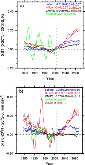
Figure 3. Time series of anomalies of (a) ASYM_SST, and (b) ASYM_PR for observations, CMIP5 LoForc (blue), CMIP5 HiForc (red) and CMIP3 (black). Observed SSTs are from Cowtan and Way (2014) (green) and reconstructed precipitation values are from Smith et al (2012) (green, 1900–2005) and 20CR (brown, 1871–2005). Observations are single realizations, whereas modelled values are ensemble means. Anomalies are calculated relative to the 1986–2005 mean. The legend gives least-squares trends and their uncertainties for 1871–2005 (or 1901–2005 for reconstructed precipitation from Smith et al) and 2006–2100 in units per century. Observational trend uncertainties are 5–95% confidence intervals, based on a t test that uses an effective sample size based on the lag-1 autocorrelation of the residuals (Santer et al 2000). Model trend uncertainties are ± one standard deviation, with each model's ensemble-mean trend taken as a data point. An 11 yr running mean has been applied to the time series before plotting.
Download figure:
Standard image High-resolution imageFigure 3(a) shows the time evolution of ensemble-mean ASYM_SST from CMIP3 and the LoForc and HiForc groups from CMIP5, for the historical period as well as the 21st century projections. Linear trends are fitted separately for 1871–2005 and 2006–2100. During the historical period, observed trends in ASYM_SST based on Cowtan and Way (2014) are not significantly different from zero (green curve); it is worth noting that ASYM_SST in the Atlantic Ocean does show a significant trend of −0.11 ± 0.08 K per century, but this is offset by changes elsewhere. Multidecadal variability is much smaller in the models than the observations, since much of it is removed by the process of ensemble averaging. Historical trends of ASYM_SST in CMIP3 (black), HiForc (red) and LoForc (blue) are within the uncertainty range of the observations and are not significantly different from zero. During the 21st century, HiForc has a significantly larger positive trend in ASYM_SST (0.25 ± 0.08 K per century) than LoForc (0.06 ± 0.07 K per century) and CMIP3 (0.05 ± 0.10 K per century). This reflects the effect of stronger radiative forcing in the NH by declining aerosols in HiForc.
The time evolution of the asymmetry index for tropical precipitation (ASYM_PR) is shown in figure 3(b). Modelled historical values of ASYM_PR show negative trends during 1871–2005, though they are only statistically significant in HiForc (−0.15 ± 0.13 mm per day per century). Reconstructed values of ASYM_PR from 20CR and Smith et al (2012) also show negative trends, with a much stronger trend in 20CR (which is also significant). The observational and statistical uncertainty makes it difficult to draw any firm conclusions regarding the realism of the modelled trends. During the 21st century, the HiForc ensemble mean shows a positive trend in ASYM_PR (0.32 ± 0.13 mm per day per century), whereas CMIP3 and LoForc have trends that are not significantly different from zero.
Modelled trends in both ASYM_SST and ASYM_PR in figure 3 are smaller in the historical period than in the projections, reflecting smaller net radiative forcing during this period, since increasing aerosols generally offset the warming influence of increasing GHGs. Compared to the other groups, CMIP5 HiForc produces the strongest trends during both periods. The historical trends are of the opposite sign to those in the projections, consistent with the reversal of aerosol emission trends from increasing to decreasing.
To what extent are trends in ASYM_PR modulated by trends in ASYM_SST on a model-by-model basis? The upper panels of figure 4 show that projected trends in ASYM_PR and ASYM_SST are highly correlated, both in CMIP3 (figure 4(a),  ) and CMIP5 (figure 4(b),
  ). In CMIP5, models in the HiForc group generally project larger trends in ASYM_PR and ASYM_SST than do models in the LoForc group. The CMIP5 HiForc models also extend further into the upper-right region of the plot, which is empty in the CMIP3 panel; thus there is a larger spread in the CMIP5 models, and the HiForc models are responsible for this.

Figure 4. Scatter plots of 2006–2100 trends in ASYM_PR versus trends in ASYM_SST: (a) CMIP3 SRESB1, (b) CMIP5 RCP4.5. In panel (b) the blue (red) symbols represent the LoForc (HiForc) group. The legend shows the correlation and level of significance, based on a two-sided t test. If FIO-ESM is excluded, the correlation increases to 0.96.
Download figure:
Standard image High-resolution imageFigure 5 shows that there are also significant correlations between trends in tropical mean precipitation and SST. This is especially true in CMIP5 projections; where the correlation between trends in tropical mean precipitation and SST exceeds 0.9. Also, the HiForc models consistently show larger trends in tropical mean precipitation and SST than the LoForc models. Importantly, figure 5 helps to put the trends in ASYM_PR in perspective: the HiForc models have ASYM_PR trends that range from roughly 0.15 to 0.6 mm per day per century, which is substantial relative to trends in tropical mean precipitation (which range from 0.01 to 0.3 mm per day per century).

Figure 5. Scatter plots of 2006–2100 trends in tropical mean precipitation versus SST, averaged over 20° S–20° N: (a) CMIP3 SRESB1, (b) CMIP5 RCP4.5. In panel (b) the blue (red) symbols represent the LoForc (HiForc) group. The legend shows the correlation and level of significance, based on a two-sided t test.
Download figure:
Standard image High-resolution imageIn summary, the HiForc projections have larger changes in the inter-hemispheric asymmetry of SST and precipitation, and larger increases in tropical mean precipitation associated with larger mean SST increases.
4. Discussion
The spatial pattern of surface-temperature response to declining aerosols is characterized by more warming in the NH than in the SH. To first order, this resembles the expected pattern of response to increasing GHGs (Stouffer et al 1989, Drost et al 2012). An important difference is that, for increasing GHGs, the radiative forcing is quasi-homogeneous in space, and the inter-hemispheric temperature asymmetry arises from feedbacks, which are mainly related to the larger land fraction in the NH (e.g., Joshi et al 2008). For aerosol changes, the feedbacks may be broadly similar, but the radiative forcing is also biased towards the NH. Thus it is perhaps not surprising that declining aerosols cause a larger inter-hemispheric asymmetry in SST and tropical precipitation than increasing GHGs. This can be inferred from our results, since there was a systematically larger inter-hemispheric asymmetry in projected tropical SST and precipitation trends in the subset of CMIP5 models with strong aerosol forcing.
Friedman et al (2013) considered changes in inter-hemispheric temperature asymmetry in historical simulations and projections forced by RCP8.5 in CMIP5 models (with a focus on hemispheric-mean surface air temperature). They found that before 1980, the GHG-forced trend in inter-hemispheric temperature asymmetry was countered by increasing aerosols, but after 1980 and through the 21st century there was a substantial increase in the (NH minus SH) temperature asymmetry. They did not consider the extent to which declining aerosols might have augmented the effects of increasing GHGs in this respect. Since the radiative forcing of increasing GHGs is very strong in RCP8.5, it is possible that the effects of declining aerosols are relatively small compared to those of increasing GHGs in this pathway. On the other hand, our results show that in projections forced by RCP4.5, declining aerosols can cause substantial, statistically significant differences between models with strong or weak aerosol forcing, and the change in sulfur dioxide emissions during the 21st century is quite similar between RCP4.5 and RCP8.5 (Bellouin et al 2011); thus the role of declining aerosols also merits investigation in RCP8.5. Note that we chose to present results based on the inter-hemispheric asymmetry in tropical SST, but broadly similar results were obtained using surface air temperature over land and ocean (not shown).
Regarding the historical period, it is interesting to compare our results with those of Hwang et al (2013), who found that CMIP3 and CMIP5 models generally underestimated the observed southward shift of tropical rainfall during the second half of the 20th century. In contrast, we did not find a significant difference between modelled and observed changes. The main reasons for the difference are likely to be (1) the different time period used in our study, and (2) the observational uncertainty. Hwang et al deliberately selected the difference of two time periods (1971–1990 minus 1931–1950), which are known to show a marked southward shift of tropical precipitation. The observed change in ASYM_PR between these periods may be enhanced by natural variability associated with the Atlantic Multidecadal Oscillation (e.g., Knight et al 2005). We showed trends for 1901–2005, which we chose as the longest period for which the reconstructed precipitation is available. The longer period is expected to smooth out some of the multidecadal natural variability. Different observational data sets were used in the two studies: whereas we used spatially complete precipitation reconstructions from 20CR and Smith et al (2012), Hwang et al used land-based observations from the Global Historical Climatology Network (GHCN) in addition to 20CR (which has markedly larger trends in ASYM_PR than the reconstruction of Smith et al). Also, whereas we considered the statistical uncertainty in the trends fitted to the reconstructed time series, Hwang et al used a single data point to represent the observed change for each reconstruction.
A possible follow-up to Hwang et al (2013) and our study would consider whether historical precipitation observations can be used to provide a top-down constraint on the precipitation response of the models. The precipitation reconstructions we used are highly uncertain over oceans, so such an analysis should preferably use high-quality precipitation data from rain gauges. Such gridded precipitation data sets include GHCN (Peterson and Vose 1997) and the Global Precipitation Climatology Centre (GPCC; Schneider et al 2014); these have limited spatial coverage, so ideally the model output would be masked to match the spatial coverage of the observations. Using such an approach, it might be possible to show that some models overestimate or underestimate the precipitation response, although the large natural variability in the observed record might limit the conclusions that can be drawn from such a comparison.
A caveat regarding the assumed decline of aerosol emissions in the 21st century is that nitrate aerosol is expected to offset declines in other aerosol species, because agricultural emissions of ammonia are assumed to be unaffected by emission controls in the RCPs (Lamarque et al 2011, Van Vuuren et al 2011). Further, nitric acid competes with sulfur dioxide for the available ammonia, so reduced emissions of sulfur dioxide, in themselves, lead to increased production of ammonium nitrate (Bellouin et al 2011). However, the only CMIP5 models that explicitly treat nitrate are the GISS-E2 models, which are excluded from our analysis (Collins et al 2013, table 12.1).
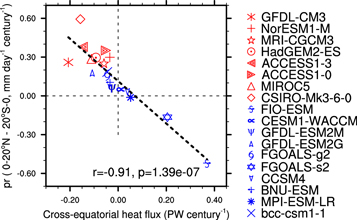
Although changes in ASYM_SST and ASYM_PR are well correlated in figure 4, an alternative energy-based perspective views changes in the latitude of tropical precipitation as a response to perturbations of the atmospheric energy balance of each hemisphere (Broccoli et al 2006, Yoshimori and Broccoli 2008, Kang et al 2009, Ming and Ramaswamy 2011, Frierson and Hwang 2012, Hwang et al 2013, Bollasina et al 2014, Bischoff and Schneider 2014, Schneider et al 2014). If energy is removed from the atmosphere of one hemisphere (say, by a change of aerosol radiative forcing), the Hadley circulation partly compensates by increasing the transport of energy into that hemisphere. Since energy is primarily transported by the upper branch of the Hadley cell, this entails a strengthening of transport in the upper branch towards the cooled hemisphere. Moisture is primarily transported by the lower branch of the Hadley cell, so tropical precipitation moves away from the cooled hemisphere. An initial energy perturbation in the midlatitudes of one hemisphere propagates to the tropics via baroclinic eddies; since temperature gradients are relatively small in the tropical free troposphere, this in turn induces a cross-equatorial energy flux (e.g., Kang et al 2009). The hemisphere from which energy is removed generally also incurs a decrease of SST (and land-surface temperature), so the viewpoints based on energy and SST are broadly consistent.
The change in (northward) cross-equatorial atmospheric energy transport is given by the integral of the change in atmospheric heating QA between 90° S and the equator or between the equator and 90° N (Frierson and Hwang 2012). Equivalently, this can be written as
where ϕ is latitude, λ is longitude and a is the radius of the Earth, and QA is calculated as the sum of the net downward radiation at the top of the atmosphere and the net upward surface energy flux. In figure 6 we plot the relationship between projected trends in  and ASYM_PR for CMIP5 (for which data availability is more complete than for CMIP3). The correlation (
 ) is similar in magnitude to that obtained between projected trends in ASYM_SST and ASYM_PR (
 ). One model (FIO-ESM) is far from the regression line in figure 4(b) and is much closer to the regression line in figure 6. However, the reverse applies for some other models (especially CSIRO-Mk3.6.0). Also, comparing figures 4(b) and 6, the demarcation between HiForc and LoForc models is less consistent for
  than for ASYM_SST. Further research is needed to achieve a complete, mechanistic understanding of the causes of meridional shifts of tropical precipitation (Schneider et al 2014).
Figure 6. Scatter plot of 2006–2100 trends in ASYM_PR versus trends in (northward) cross-equatorial atmospheric energy transport in CMIP5 projections forced by RCP4.5. The legend shows the correlation and level of significance, based on a two-sided t test. Two models (CESM1-CAM5-1-FV2 and EC-EARTH) were omitted due to lack of flux data.
Download figure:
Standard image High-resolution image
5. Conclusions
Our results show that assumptions about aerosol emissions and indirect aerosol effects exert a strong influence on the magnitude and pattern of projected tropical precipitation and SST change: models in the CMIP5 HiForc group consistently project larger changes in both the mean and north–south asymmetry of tropical precipitation and SST than do models in the LoForc group. Earlier projections from CMIP3 (forced by the SRES B1 scenario) behave more like the LoForc group, probably due to a combination of two factors: (1) future aerosol declines are assumed to be smaller in the SRES scenarios than in the RCPs; (2) only two of 20 CMIP3 models treat indirect effects of aerosols on both cloud albedo and cloud lifetime (the criterion that defines the CMIP5 HiForc group). The latter point suggests that aerosol forcing tends to be weaker in CMIP3 models than in the CMIP5 HiForc group, although information about aerosol ERF in CMIP3 is generally unavailable.
It follows that anthropogenic aerosols need to be considered as an important source of scatter in models' projected changes of tropical precipitation. This is likely to be especially true in the lower forcing pathways, since then changes in aerosol forcing represent a larger fraction of the total forcing. If the real world resembles the HiForc group, then future aerosol changes are likely to be an important (even dominant) driver of tropical precipitation changes under low to moderate forcing scenarios. Near-term aerosol changes may also be an important source of skill for near-term climate projections (Kirtman et al 2013, Bellucci et al 2015), especially if the real world is more like the HiForc group than the LoForc group. Since CO2 forcing does not vary significantly across the RCPs on a 20 to 30 year time horizon (even under aggressive mitigation), changes in aerosol forcing may be the primary driver of forced precipitation changes on these timescales, but they are also a large source of uncertainty.
The 20 CMIP5 models that we examined do not capture the full uncertainty range of historical aerosol ERF, which ranges from −0.1 to −1.9 W m−2 in the global mean (Boucher et al 2013). Taking this into account, as well as uncertainty regarding whether aerosol declines projected under the RCPs are achievable, the total uncertainty caused by aerosols may be even larger than indicated here. The models in the HiForc group have aerosol ERF that is stronger than the best estimate from Boucher et al (2013), and it is possible that they overestimate the magnitude of aerosol effects. Efforts should continue to constrain the magnitude of aerosol forcing, in order to reduce the uncertainty of possible aerosol-driven changes in future tropical precipitation and SST.
Acknowledgments
This research is partly supported by the Australian Government Department of the Environment, the Bureau of Meteorology and CSIRO through the Australian Climate Change Science Programme. We acknowledge the World Climate Research Programme's Working Group on Coupled Modelling and the US Department of Energy's Program for Climate Model Diagnosis and Intercomparison, and we thank the climate modeling groups (listed in tables 1 and 2 of this paper) for producing and making available their model output. We thank Tim Cowan and two anonymous referees for their helpful comments on the manuscript, and Yi Ming for providing additional output from the GFDL-CM3 model.