
Topological objects in field theory
Published November 2019
•
Copyright © 2019 Morgan & Claypool Publishers
Pages 8-1 to 8-28
You need an eReader or compatible software to experience the benefits of the ePub3 file format.
Download complete PDF book, the ePub book or the Kindle book

Permissions
Abstract
In this chapter, I present an overview of topological objects in quantum field theory. I start with the Sine-Gordon model and then present topogolical solutions for gauged complex fields and Yang-Mills theory. Finally, I discuss quantum anomalies and their relation to topology.
In non-linear classical field theories there can exist stable configurations with well-defined energy, which are solutions to the classical equations of motion, but which possess some special properties such as propagation without dissipation. For example, the sine-Gordon model possesses solitonic solutions. Since non-abelian gauge theory is non-linear, there may exist important topological solutions such as vortices, monopoles, and 'instantons' that are soliton-like solutions.
8.1. The kinky sine-Gordon model
The 1+1d 'sine-Gordon' equation of motion is

which describes a scalar field in one space and time dimension in a periodic potential. The corresponding Lagrangian is

and the Hamiltonian density is

with

We have plotted this potential in figure 8.1. As we can see from this figure, there are an infinite number of stable degenerate 'vacuum' solutions given by


Figure 8.1. Sine-Gordon potential.
Download figure:
Standard image High-resolution imageSuch trivial static solutions have zero energy
 and all non-trivial solutions we obtain below
will only be defined up to a shift by
and all non-trivial solutions we obtain below
will only be defined up to a shift by
 . As we will see, there are solutions to these
equations that allow us to connect the different degenerate minima.
. As we will see, there are solutions to these
equations that allow us to connect the different degenerate minima.
Note that, if we were to treat this problem perturbatively, we would expand equation (8.4)

which looks like a
potential for a particle with mass
 and coupling
 .
.
We begin by looking for static solutions with
 , and hence need to solve

Multiplying left and
right by  and simplifying gives

Integrating, gives

We will search for solutions that have
 at both
 and
and
 and
and
 for
for
 and
and
 , respectively. This implies that
 , giving

and hence

Separating and integrating, we obtain

This gives

with
 being an integration constant. Solving for
 , we obtain

The kink
(+) and anti-kink (−) solutions are plotted figure 8.2 left panel. In the right panel of the same
figure we show a visualization of field rotation associated with the kink solution. As
can be seen from this figure, the kink solution moves from a vacuum state with
 to one with
 . The kink is topological in
the sense that one cannot continuously deform the right panel of figure 8.2 while keeping the final
vectors the same and get rid of the kink (rotation in the phase vector). The anti-kink
is similar but instead moves one from
. The kink is topological in
the sense that one cannot continuously deform the right panel of figure 8.2 while keeping the final
vectors the same and get rid of the kink (rotation in the phase vector). The anti-kink
is similar but instead moves one from
 to
to
 . Classically, these solutions are ones in
which the system starts asymptotically at one minimum and reaches the other minimum at
large times.
. Classically, these solutions are ones in
which the system starts asymptotically at one minimum and reaches the other minimum at
large times.

Figure 8.2. (Left) Kink and anti-kink sine-Gordon solutions for
 and
and
 . (Right) Visualization of the phase
rotation associated with the kink solution.
. (Right) Visualization of the phase
rotation associated with the kink solution.
Download figure:
Standard image High-resolution imageIn the non-stationary case, we search for solutions of the form
 with
with
 . Plugging this ansatz into the sine-Gordon
equation gives
. Plugging this ansatz into the sine-Gordon
equation gives

with
 and
and
 . This looks exactly like equation (8.7), so we can take
the solution directly over to obtain
. This looks exactly like equation (8.7), so we can take
the solution directly over to obtain

This solution represents a kink (or anti-kink) moving at finite velocity. It has a finite energy, which can be computed from the integral of the Hamiltonian density. Since adding the time dependence just gives a moving kink, it suffices to consider the energy of a static kink
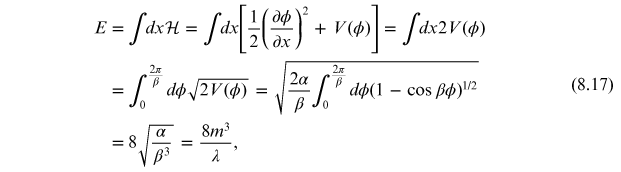
where we used equations
(8.10) and
(8.11) and, in
the last line, we re-expressed the energy in terms of the mass and coupling constant
introduced in equation (8.6). This shows that the energy of the kink solution is finite and,
importantly, that the energy goes inversely with the coupling
 meaning that, in the strong coupling limit,
the energy associated with such configurations can become small.
meaning that, in the strong coupling limit,
the energy associated with such configurations can become small.
We note that similar non-trivial solutions can be obtained by assuming that
 can be expressed in the form [1]

For example, for
 , there is a two-kink solution of the
form
, there is a two-kink solution of the
form

This solution is plotted
and visualized in figure 8.3 for the case
 at
at
 .
.

Figure 8.3. (Left) Two-kink sine-Gordon solution for
 . (Right) Visualization of the phase
rotation associated with the two-kink solution. For both panels we took
. (Right) Visualization of the phase
rotation associated with the two-kink solution. For both panels we took
 and
and
 .
.
Download figure:
Standard image High-resolution imageIn fact, a family of solutions with an arbitrary number of kinks + anti-kinks can be constructed in this manner. Each of these solutions has a conserved number associated with the number of kinks minus anti-kinks. One can construct a conserved current of the form

with
 and
and
 being the 1+1 anti-symmetric tensor with
 . This current is conserved, that is
 , and the conserved charge associated with it
is
, and the conserved charge associated with it
is

where
 can be identified as the difference of the
number of kinks minus anti-kinks. From this we see the important role played by the
boundary conditions at infinity. The (anti)-kink and two-kink solutions presented
earlier in this section have charge
can be identified as the difference of the
number of kinks minus anti-kinks. From this we see the important role played by the
boundary conditions at infinity. The (anti)-kink and two-kink solutions presented
earlier in this section have charge
 and 2, respectively. Note that the solitonic
current is not a Noether current associated with a global symmetry, it instead comes
from the conservation of 'winding number', which is a topological invariant.
and 2, respectively. Note that the solitonic
current is not a Noether current associated with a global symmetry, it instead comes
from the conservation of 'winding number', which is a topological invariant.
8.2. Two-dimensional vortex lines
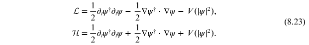
Next we consider a complex scalar field (charged scalar) in two spatial dimensions. We
take the boundary of space to be the circle at infinity,
 . We will impose a boundary condition at
infinity
. We will impose a boundary condition at
infinity

where
 and
and
 are polar coordinates in the plane,
 is an arbitrary amplitude, and
 is an integer in order to guarantee that
 is single valued.
The Lagrangian and Hamiltonian densities are
As our example, let us
take
 such that
 at the boundary.
To start with, let us consider a static configuration. In this case, the Hamiltonian density at the boundary is

Since the Hamiltonian
density only falls off like
 , this implies that the energy of such a
configuration is infinite. This means that there is no finite-energy generalization of
the 1d kink solution for a 2d complex scalar.
, this implies that the energy of such a
configuration is infinite. This means that there is no finite-energy generalization of
the 1d kink solution for a 2d complex scalar.
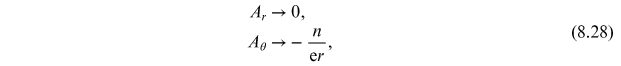
Next, let us consider what happens if we couple our complex scalar field to an abelian
gauge field by taking
 with
with

and require that the vector potential has the boundary condition

As we demonstrate below, by adding a gauge field with these non-trivial boundary conditions, one can construct a discrete set of finite-energy configurations of a complex scalar coupled to an abelian gauge field. Including the gauge-field contribution to the Lagrangian density, we have

To see that the energy of a configuration satisfying equations (8.22) and (8.26) is finite, we
first note that, given the boundary condition for
 above, one has
which implies that, at asymptotically large distances, one has
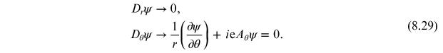
This means
 falls faster than
 at infinity and the kinetic energy
contribution will be UV finite. Additionally, since equation (8.26) can be
expressed in the form
at infinity and the kinetic energy
contribution will be UV finite. Additionally, since equation (8.26) can be
expressed in the form
 with
with
 , this gauge field is a pure gauge
transform and carries zero energy. As a result, all terms in equation (8.27) result in a
finite contribution to the total energy.
, this gauge field is a pure gauge
transform and carries zero energy. As a result, all terms in equation (8.27) result in a
finite contribution to the total energy.
The gauge field configuration possesses a quantized magnetic flux. To
see this, consider the magnetic flux
 generated by equation (8.28) through a disk
of radius
generated by equation (8.28) through a disk
of radius  with boundary


which shows that the flux is quantized. We have demonstrated that it is possible to construct a 2d configuration consisting of a charged scalar field plus a gauge field that carries a quantized magnetic flux.
This 2d solution can be extended to 3d by simplying requiring cylindrical symmetry of
the 3d system. In this case, the quantized flux lines are the 'Abrikosov flux lines'
which appear in the theory of type II superconductors. The model we analyzed (8.23) corresponds to
scalar electrodynamics with spontaneous symmetry breaking (Higgs model). This is a
relativistic generalization of the condensed matter field theory, with the field
 corresponding to the
Bardeen-Cooper-Schrieffer condensate. In a type II superconducting medium, the magnetic
field normally cannot penetrate the material and if it does, it can only do so through
quantized flux lines called Abrikosov flux lines. For a more extensive
discussion of topological solutions in the context of condensed matter see ref. [2].
corresponding to the
Bardeen-Cooper-Schrieffer condensate. In a type II superconducting medium, the magnetic
field normally cannot penetrate the material and if it does, it can only do so through
quantized flux lines called Abrikosov flux lines. For a more extensive
discussion of topological solutions in the context of condensed matter see ref. [2].
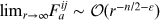
8.3. Topological solutions in Yang–Mills
The next question one naturally asks is whether it is possible to construct analogous classical Yang–Mills topological solutions. To determine whether such non-abelian topological solutions are possible, we ask if it is possible to construct finite-energy classical solutions with non-trivial boundary conditions. We specialize to the case of pure-gauge fields, in which case the canonical energy momentum tensor is expressible solely in terms of the field-strength tensor (see volume 1)

which obeys

The energy-momentum tensor is gauge-invariant. From equation (8.31) we have

where
 is the number of spatial dimensions.
8.3.1. Static solutions
Topological solutions can be time-dependent or time-independent (static). A static
solution is one where
 can be made time-independent using a
continuous gauge transformation. For such static solutions, the general time evolution
of
can be made time-independent using a
continuous gauge transformation. For such static solutions, the general time evolution
of  can be obtained from a continuous gauge
transformation
can be obtained from a continuous gauge
transformation

where
 is an arbitrary continuous function. We can
make the right-hand side vanish if
is an arbitrary continuous function. We can
make the right-hand side vanish if

which is solved by

with
 being the gauge-link,
which is the exponential of the integral of the gauge potential along the path
being the gauge-link,
which is the exponential of the integral of the gauge potential along the path


In the definition of
 ,
,
 implies the path-ordering
operator, which orders
implies the path-ordering
operator, which orders
 similar to the time-ordering operator, but
now for a path in space-time.
similar to the time-ordering operator, but
now for a path in space-time.
With  determined in this way, we have
 , that is the field configuration is
time-independent. The gauge in which our static field is time-independent is called
the static gauge. Static solutions with finite-energy are either the
vacuum or a static solution. For pure Yang–Mills theory it turns out that there are no
static topological solutions unless the number of spatial dimensions is four [3]. We will now review the
proof of this statement by considering Yang–Mills in
, that is the field configuration is
time-independent. The gauge in which our static field is time-independent is called
the static gauge. Static solutions with finite-energy are either the
vacuum or a static solution. For pure Yang–Mills theory it turns out that there are no
static topological solutions unless the number of spatial dimensions is four [3]. We will now review the
proof of this statement by considering Yang–Mills in
 dimensional Minkowski space.
The requirement of finite-energy implies that

One can show that, for
a static solution,
 with i = 1, 2, 3
(homework), and hence one has
with i = 1, 2, 3
(homework), and hence one has

As a result,
 with
with
 and
and
 and one must have
 for convergence in the UV.
Next, consider

Since
 , one has
 , giving

For a static solution, the second term vanishes, leaving

Integrating on the left
and right we see that, since
 vanishes at infinity, the integral of the
left-hand side has to vanish and, therefore, so does the integral over the right-hand
side
vanishes at infinity, the integral of the
left-hand side has to vanish and, therefore, so does the integral over the right-hand
side

Using
 , equation (8.33), and
 we obtain

Therefore, unless
 one must have
 everywhere for this integral to be zero
(integrand is positive-definite). We thus conclude that for
everywhere for this integral to be zero
(integrand is positive-definite). We thus conclude that for
 there cannot be static pure-gauge
topological solutions. For
there cannot be static pure-gauge
topological solutions. For
 we can find a solution, which is called the
instanton solution. We will construct such a solution next.
we can find a solution, which is called the
instanton solution. We will construct such a solution next.
8.4. The instanton
A static topological solution in 4 + 1 Minkowski space is a time-independent solution
that only depends on the four-dimensional Euclidean space coordinates. Since we can
formulate the path integral in four-dimensional Euclidean or Minkowski spaces, a
four-dimensional Euclidean solution might be of some interest. As an example, let us
search for a solution that is invariant under
 gauge transformations with
 . What we are looking for is a mapping from
the
. What we are looking for is a mapping from
the  group space
 to the boundary of the physical space, which
is also
to the boundary of the physical space, which
is also  .
.
We will label Euclidean space with spatial coordinates
 . The Euclidean field tensor
 is defined in the same way as the Minkowski
tensor
is defined in the same way as the Minkowski
tensor

Defining
 and
and
 we can write this compactly as
![${F}_{\mu \nu }={\partial }_{\mu }{A}_{\nu }\,-{\partial }_{\nu }{A}_{\mu }-ig[{A}_{\mu },{A}_{\nu }]$](https://content.cld.iop.org/books/10__1088_2053-2571_ab3108/revision2/bk978-1-64327-708-0ch8ieqn139.gif) . We can introduce the dual
of
. We can introduce the dual
of  as
as
 which is defined by

where, since we are in Euclidean space, we do not have to distinguish up and down indices.
We can express

with

being the
Chern–Simons current. Since
 can be expressed as a total derivative of the
Chern–Simons current, its integral can only depend on the boundary conditions for the
current. Considering a four-dimensional Euclidean volume
can be expressed as a total derivative of the
Chern–Simons current, its integral can only depend on the boundary conditions for the
current. Considering a four-dimensional Euclidean volume
 with boundary
 . Suppose that on the boundary we have a pure
vacuum solution with
. Suppose that on the boundary we have a pure
vacuum solution with
 ,
,
 , and, hence,
 . In the absence of matter, the equation of
motion for the field in the entire volume
. In the absence of matter, the equation of
motion for the field in the entire volume
 is
is

Additionally, the dual satisfies

which follows from the
Bianchi identity. Using the current
 , we can write

where
 is the projection of
 that is perpendicular to the surface
 . Note that this is trivially satisfied if the
solution is pure vacuum everywhere in
. Note that this is trivially satisfied if the
solution is pure vacuum everywhere in
 .
.
To proceed, we imagine performing a space-time dependent gauge transformation on the
boundary 

Since the result is a
pure-gauge field, one still has
 on the boundary, but it may be possible to
have
on the boundary, but it may be possible to
have  .
.
Choosing

with
 gives
gives


and

Using this, we obtain

We see from this
expression that although
 vanishes on the boundary at infinity, it
cannot be zero everywhere within
vanishes on the boundary at infinity, it
cannot be zero everywhere within
 since the integral above is finite. This
means that the solution cannot be a pure gauge everywhere in
since the integral above is finite. This
means that the solution cannot be a pure gauge everywhere in
 . We will return to this issue
shortly.
. We will return to this issue
shortly.
Exercise 8.1 Show that equation (8.48) is correct.
Exercise 8.2 Show that equation (8.50) is correct.
Exercise 8.3 Show that equations (8.54) and (8.55) are correct.
8.5. The Potryagin index
The quantity introduced above
 is related to the Potryagin
or topological index, which is denoted as
is related to the Potryagin
or topological index, which is denoted as
 ,
,

The vacuum has
 . Equation (8.53) gives
 according to equation (8.57).
We will now show that  is the degree of the mapping of the group
space from the spatial coordinate boundary (number of times it covers the group space).
In this case we have a mapping of
is the degree of the mapping of the group
space from the spatial coordinate boundary (number of times it covers the group space).
In this case we have a mapping of
 , which is the group space of
 , onto a
 in coordinate space. Computing
 using equations (8.48) and (8.52) one
obtains
using equations (8.48) and (8.52) one
obtains

This allows us to express
 as
as
where
 is an outward pointing unit vector. To
proceed, let us consider a parameterization of the
is an outward pointing unit vector. To
proceed, let us consider a parameterization of the
 using parameters
 . With this we have
From the last line, we
learn that  is the number of times that the group space
is covered by the map the coordinate
is the number of times that the group space
is covered by the map the coordinate
 to the group
 . This is sometimes called the 'winding
number' of the map.
. This is sometimes called the 'winding
number' of the map.
As a simpler example of this, let us look at a map from
 to
to
 using a
 configuration of the form

where
 with
with
 covering the circle. Requiring that
 be singled-valued for
 we see that
 where
where
 . The corresponding pure-gauge vector
potential constructed from this is
. The corresponding pure-gauge vector
potential constructed from this is

One, therefore, has

where
 is the winding number, which
counts the number of times
is the winding number, which
counts the number of times
 goes around the
 circle when
 runs around the
 circle once
 . This is similar to the phase we accumulated
in the sine-Gordon model when we made a transition from one vacuum to another. The
situation is similar in pure-gauge QCD, the mapping of
. This is similar to the phase we accumulated
in the sine-Gordon model when we made a transition from one vacuum to another. The
situation is similar in pure-gauge QCD, the mapping of
 generates a topologically conserved number,
which is the Potryagin index of the field configuration.
generates a topologically conserved number,
which is the Potryagin index of the field configuration.
Exercise 8.4 Derive equation (8.59).
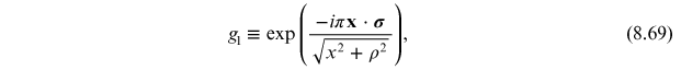
8.6. Explicit solution for a q = 1 instanton
As mentioned previously, the field cannot be a pure-gauge configuration everywhere if
 is non-zero. The instanton solution in all of
 is
1
is
1

where
 and
and
 is an arbitrary real constant which sets the
size of the instanton solution. As
is an arbitrary real constant which sets the
size of the instanton solution. As
 this solution reduces to the pure-gauge form
given by equation (8.52). Generally, one has
this solution reduces to the pure-gauge form
given by equation (8.52). Generally, one has


The asymptotic form of this solution can be obtained from gauge transformations of the type

with
and

The gauge transform
 is an element of
 but
but
 and
and
 for
for
 are not homotopic, that is
they have a different topology and cannot be continuously deformed into one another. The
are not homotopic, that is
they have a different topology and cannot be continuously deformed into one another. The
 instanton configuration describes a solution
of the gauge-field equations in which, as
instanton configuration describes a solution
of the gauge-field equations in which, as
 goes from
 to
to
 , a vacuum belonging to homotopy
class
, a vacuum belonging to homotopy
class
 evolves into another vacuum with homotopy
class
evolves into another vacuum with homotopy
class  . The energy density of the pure-gauge field
at the end-point is vanishing, however, the full configuration has a positive field
energy. As a result, we see that the Yang–Mills vacuum is infinitely degenerate with an
infinite number of homotopically non-equivalent vacua. The instanton represents a
transition from one vacuum class to another. Due to the finite energy of the instanton,
classically there can be no transition between the degenerate vacua, however, quantum
mechanically we have the possibility of quantum tunneling.
. The energy density of the pure-gauge field
at the end-point is vanishing, however, the full configuration has a positive field
energy. As a result, we see that the Yang–Mills vacuum is infinitely degenerate with an
infinite number of homotopically non-equivalent vacua. The instanton represents a
transition from one vacuum class to another. Due to the finite energy of the instanton,
classically there can be no transition between the degenerate vacua, however, quantum
mechanically we have the possibility of quantum tunneling.
8.7. Quantum tunneling, θ-vacua, and symmetry breaking
The barrier potential amplitude is given
 where
where
 is the Euclidean action. To see this,
consider the motion of a particle with energy
is the Euclidean action. To see this,
consider the motion of a particle with energy
 in a one-dimensional potential
 in the WKB approximation. If
 , the transition is classically forbidden, and
the quantum tunneling amplitude is
, the transition is classically forbidden, and
the quantum tunneling amplitude is

where we have identified
the Euclidean action  with the integral appearing on the left. Let
us see why this is true. If
with the integral appearing on the left. Let
us see why this is true. If
 , the transition is classically allowed and
the wave function oscillates with the number of oscillations given by
, the transition is classically allowed and
the wave function oscillates with the number of oscillations given by

Alternatively, we can
express the integral of  as
as

If the total energy is normalized to zero which it always can be, then

This is the total action
induced transversing from  to
to
 .
.
The only difference between the classically forbidden case and the allowed case just
considered, is the sign of  and, since we have normalized the energy such
that
and, since we have normalized the energy such
that  , we see that we simply pick up a relative
factor of
, we see that we simply pick up a relative
factor of  from the square root. The sign of
 in the classical equation of
motion
in the classical equation of
motion

is reversed if we take
 . As a result,
 is the action for imaginary times. This
justifies calling
is the action for imaginary times. This
justifies calling
 the tunneling amplitude.
Now we need to determine the action for our instanton. For this we need to be able to evaluate

The
 solution given in equation (8.65) is special
because it is self-dual meaning that
solution given in equation (8.65) is special
because it is self-dual meaning that

As a result,

For the
 instanton constructed herein, this gives a
transition probability of
instanton constructed herein, this gives a
transition probability of
 and in general, one finds,
 . For small
 , such transitions are extremely strongly
suppressed. Regardless of the magnitude of
, such transitions are extremely strongly
suppressed. Regardless of the magnitude of
 , however, the fact that these tunneling
solutions exist means that all of the degenerate vacua of Yang–Mills are coupled by
instantons.
, however, the fact that these tunneling
solutions exist means that all of the degenerate vacua of Yang–Mills are coupled by
instantons.
We can label each of the generate vacuum by the topological index which must be an
integer, so we have a basis of states of the form
 with
with
 . Positive
 map to multi-instanton solutions with more
instanton than anti-instanton solutions and vice-verse for negative
map to multi-instanton solutions with more
instanton than anti-instanton solutions and vice-verse for negative
 and
and
 is the instanton-free vacuum. The true wave
function of the QCD vacuum is therefore a linear superposition of states, however, since
instantons couple the various vacuum states, we must diagonalize the Hamiltonian to
obtain the true ground state. The end result is that the QCD vacuum will have the
form
is the instanton-free vacuum. The true wave
function of the QCD vacuum is therefore a linear superposition of states, however, since
instantons couple the various vacuum states, we must diagonalize the Hamiltonian to
obtain the true ground state. The end result is that the QCD vacuum will have the
form

where
 is an arbitrary constant. This is vacuum is
called the theta vacuum. The form of the coefficients in this expansion
guarantee that the
is an arbitrary constant. This is vacuum is
called the theta vacuum. The form of the coefficients in this expansion
guarantee that the  -vacuum is invariant under gauge
transformations of the type
-vacuum is invariant under gauge
transformations of the type
 . Acting with
 we find

and hence the theta vacuum simply picks up a phase

Although one can
construct stationary states for any value of
 , they are not excitations of the
 vacuum, because in QCD the value of
 cannot be changed. As far as the strong
interaction is concerned, different values of
cannot be changed. As far as the strong
interaction is concerned, different values of
 correspond to different worlds. We can fix
the value of
correspond to different worlds. We can fix
the value of  by adding an additional term of the
form
by adding an additional term of the
form

to the QCD Lagrangian.
Does physics depend on the value of
 ? The interaction above violates both T and CP
invariance. On the other hand, it is a surface term and it might be possible that
confinement somehow screens the effects of the
? The interaction above violates both T and CP
invariance. On the other hand, it is a surface term and it might be possible that
confinement somehow screens the effects of the
 -term. A similar phenomenon is known to occur
in three-dimensional compact electrodynamics. In QCD, however, one can show that, if the
-term. A similar phenomenon is known to occur
in three-dimensional compact electrodynamics. In QCD, however, one can show that, if the
 problem is solved (there is no massless
 state in the chiral limit) and none of the
quarks are massless, a non-zero value of
state in the chiral limit) and none of the
quarks are massless, a non-zero value of
 implies that CP symmetry is broken [5–8]. The most severe limits on CP violation in
the strong interaction come from the electric dipole of the neutron. Current experiments
imply that
implies that CP symmetry is broken [5–8]. The most severe limits on CP violation in
the strong interaction come from the electric dipole of the neutron. Current experiments
imply that
 [9, 10]. The question of why
 is so small is known as the strong CP
problem.
is so small is known as the strong CP
problem.
Exercise 8.5 Show that equation (8.77) is obeyed by a
 instanton solution.
8.8. Quantum anomalies
It is possible that classical symmetries of a system do not survive quantization, in which case it is said that the theory possesses a quantum anomaly. If this is case, the Noether current associated with the classical symmetry is no longer conserved after quantization and the current conservation law is said to receive an anomalous contribution. This is relevant for this course because QCD has a chiral anomaly, which is associated with the non-conservation of the chiral current in the limit of vanishing light quark masses. This will be the focus of the remainder of the chapter.
Historically, the reaction
 is the best example of a process that
proceeds primarily via the chiral anomaly. The original calculation of this anomalous
decay was performed in 1969 by Bell and Jackiw and, independently, Adler. As a result,
it is sometimes referred to as the Adler-Bell-Jackiw (ABJ) anomaly
[11–13]. Earlier calculations of
the
is the best example of a process that
proceeds primarily via the chiral anomaly. The original calculation of this anomalous
decay was performed in 1969 by Bell and Jackiw and, independently, Adler. As a result,
it is sometimes referred to as the Adler-Bell-Jackiw (ABJ) anomaly
[11–13]. Earlier calculations of
the
 decay width, which did not take into chiral
anomaly, resulted in a decay lifetime on the order of 10−33 s, which was
approximately three orders of magnitude longer than the experimentally observed pion
lifetime. As of the 2015 PDG listings, the pion lifetime is
decay width, which did not take into chiral
anomaly, resulted in a decay lifetime on the order of 10−33 s, which was
approximately three orders of magnitude longer than the experimentally observed pion
lifetime. As of the 2015 PDG listings, the pion lifetime is
 . The branching ratio for the
 decay channel is
 and hence it dominates the total lifetime
calculation for the pion. Taking into account the chiral anomaly, ABJ obtained a decay
width of
and hence it dominates the total lifetime
calculation for the pion. Taking into account the chiral anomaly, ABJ obtained a decay
width of
 . This maps to a total pion lifetime of
approximately
. This maps to a total pion lifetime of
approximately
 , which is in the right ballpark and, within
the modern experimental error bars
2
.
, which is in the right ballpark and, within
the modern experimental error bars
2
.
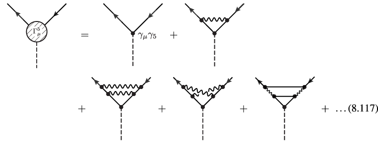
In perturbation theory, one can understand the emergence of the chiral anomaly through the consideration of triangle graphs of the form
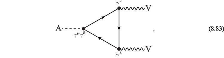
where A stands for 'axial' and V stands for 'vector'. Such graphs naturally arise in the calculation of the pion decay rate. There are also VVV graphs and other configurations that occur at higher orders, however, it turns out that once we understand the anomaly in the AVV graph it is automatically handled in all of the other graphs. Before proceeding to this technical calculation, however, I would first like to discuss the physics of the anomaly.
8.8.1. The chiral anomaly in the Schwinger model
The Schwinger model is simply 1+1d massless QED. The Lagrangian density is

where, as usual,
 is the covariant derivative and the
 Dirac matrices can be written in terms of
the Pauli matrices
Dirac matrices can be written in terms of
the Pauli matrices

The resulting classical equations of motion are


where

is the conserved vector
current,
 . This conserved current results from the
local gauge invariance of the Schwinger model and QED in general.
. This conserved current results from the
local gauge invariance of the Schwinger model and QED in general.
There is also an axial current or chiral current

where
 . This chiral current is classically
conserved
. This chiral current is classically
conserved
 and this conservation law is associated
with classical invariance of QED under global chiral transformations
of the fermionic fields
and this conservation law is associated
with classical invariance of QED under global chiral transformations
of the fermionic fields

We can identify the two components of the spinor as 'left'- and 'right'-handed

where
 with
with
 being a left/right projector. Under a
chiral transformation the left and right fields pick up opposite phases
being a left/right projector. Under a
chiral transformation the left and right fields pick up opposite phases

Expanding out the free
fermionic contribution to the Lagrangian in terms of
 , we obtain

and the general solution to the equations of motion in this case will be of the form
This demonstrates that,
in the Schwinger model, left- and right-handed particles are quite literally left- and
right-moving particles. This is different than the 3+1d case where chirality is
related to the alignment of the particle's spin with its momentum (helicity). In 1+1d,
there is no spin and the handedness is related to particles propagating either to the
left and right. This only makes sense in the massless case where particles move at the
speed of light and the direction of propagation is the same in all reference frames.
In addition, in this case we see that a parity transformation
 transforms left-movers into right-movers.
This will be become important since, if the symmetry between left- and right-movers is
broken, then we might break parity symmetry.
transforms left-movers into right-movers.
This will be become important since, if the symmetry between left- and right-movers is
broken, then we might break parity symmetry.
We also see that the free part of the Lagrangian is invariant under chiral transformations (8.92) since left- and right-handed fields only couple to themselves. The same holds for the interaction part, where one finds

Note that, in the
classical theory, the number of left- and right-handed fermions,
 and
and
 , are independent constants of the motion.
This will remain true if the fermions are coupled to a gauge field.
, are independent constants of the motion.
This will remain true if the fermions are coupled to a gauge field.
8.8.2. Understanding the anomaly
Before proceeding more formally, let us consider what would happen if we apply an
external electric field
 to a system of positively charged particles
for a short amount of time
to a system of positively charged particles
for a short amount of time
 . In this case, the right-movers will gain
energy
. In this case, the right-movers will gain
energy

and left-movers will
lose the same amount of energy. If the initial state before the electric field was
turned on is the Dirac vacuum, with all negative energy levels filled, then after the
time interval
 , the right-handed 'Fermi-level' has
increased by
, the right-handed 'Fermi-level' has
increased by
 and the left-handed Fermi level has
decreased by
and the left-handed Fermi level has
decreased by
 . As a result, right-handed fermions are
created along with left-handed anti-fermions (holes). This is sketched in figure 8.4.
. As a result, right-handed fermions are
created along with left-handed anti-fermions (holes). This is sketched in figure 8.4.

Figure 8.4. Action of an external electric field on left- and right-movers. Grey lines represent the filled fermion levels.
Download figure:
Standard image High-resolution imageSince the one-dimensional density of states is
 , the number density per unit length of
left- and right-handed fermions become
, the number density per unit length of
left- and right-handed fermions become

Therefore, the 'vector' fermion number associated with charge conservation is conserved during this process

however, the 'axial' fermion number, which is also conserved at the classical level, changes according to

The fact that the right hand side is non-vanishing is the chiral anomaly. The chiral anomaly corresponds to a kind of dielectric breakdown of the vacuum where we create particle-hole pairs with a chiral imbalance.
At this point, you should be scratching your head in confusion since everything we
just did was classical; however, the subtlety in the argument is the existence of an
infinitely occupied Dirac sea in the first place. Imagine that instead of an infinite
number of negative energy states, there were a finite number of them, regulated by a
cutoff  on the lowest possible negative energy
state before turning on the electric field. In that case, figure 8.4 would look instead like figure 8.5 and we would always have
the same number of left- and right-moving states even in the presence of an external
electric field. As a result, we see that the physics of the anomaly will be tied
intimately with the regularization of the theory. If we regularize and do not remove
the regulator, we might even miss it! Note that, if you hear condensed matter
theorists discussing the chiral anomaly, the figure they use to illustrate the concept
will look more like figure 8.6.
on the lowest possible negative energy
state before turning on the electric field. In that case, figure 8.4 would look instead like figure 8.5 and we would always have
the same number of left- and right-moving states even in the presence of an external
electric field. As a result, we see that the physics of the anomaly will be tied
intimately with the regularization of the theory. If we regularize and do not remove
the regulator, we might even miss it! Note that, if you hear condensed matter
theorists discussing the chiral anomaly, the figure they use to illustrate the concept
will look more like figure 8.6.

Figure 8.5. In this case, we imagine that the Dirac sea is not an infinite reservoir, but is instead finite.
Download figure:
Standard image High-resolution image
Figure 8.6. An alternative visualization of the chiral anomaly. The left panel shows the vacuum before the electric field is applied and the right panel shows after. Closed circles indicate filled states and open unfilled states. Diagonal lines are the light cones along which the massless fermions propagate.
Download figure:
Standard image High-resolution image
8.8.3. The chiral anomaly in 3+1d
The natural followup question is, of course, if this kind of logic can be extended to
3+1d. As it turns out, the precise discussion we just had applies in 3+1d to massless
fermions in a magnetic field. This is because fermions in a background magnetic field
are restricted to Landau levels labeled by an integer
 [17]. For massless fermions, the Landau
levels are
[17]. For massless fermions, the Landau
levels are

where
 is an integer,
 , and
, and
 . The fermionic motion in the
 plane is quantized circular motion and the
fermions effectively propagate along the z-axis like 1+1d fermions
with mass
plane is quantized circular motion and the
fermions effectively propagate along the z-axis like 1+1d fermions
with mass

For a positively
charged particle,  , with
 , we see that the lowest Landau level
 the effective mass vanishes and, hence,
these particles will behave like massless 1+1d fermions. For a negatively charged
particle, we have the same behavior for the
the effective mass vanishes and, hence,
these particles will behave like massless 1+1d fermions. For a negatively charged
particle, we have the same behavior for the
 .
.
For massless 3+1d fermions, chirality is identified with the helicity of the state.
The right-handed fermion with
 is a right-mover along the
z-axis and the left-handed fermion is a left-mover. So, by adding a
background field, at least some subset of the allowed states are effectively 1+1 and
our previously setup can be applied. We now imagine applying an electric field along
the
is a right-mover along the
z-axis and the left-handed fermion is a left-mover. So, by adding a
background field, at least some subset of the allowed states are effectively 1+1 and
our previously setup can be applied. We now imagine applying an electric field along
the  direction,
 , and our earlier discussion applies. The
density of states per unit area in a Landau level is
, and our earlier discussion applies. The
density of states per unit area in a Landau level is

therefore, axial charge is created at a rate of

where now the right-hand side indicates the presence of a 3+1d axial anomaly. Stated succinctly, an electric field applied to the vacuum causes pair production and, if a parallel magnetic field is applied, the pairs created are chiral. Positively-charged fermions will align their spins with B, while anti-fermions (negative charge in this case), anti-align their spins with B 3 .
We would like to express
 in terms of the axial (chiral) charge

and the contraction of the field strength tensor and the dual field strength tensor

where we remind you
that
 . This gives

This is the standard way to present the anomalous contribution, which breaks chiral current conservation.
Exercise 8.7 Derive equation (8.99).
Exercise 8.8 Derive equation (8.104).
8.9. An effective Lagrangian for the anomaly
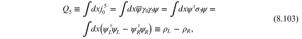
Now that we have a kind of intuitive understanding of the phenomenon, let us return to the mathematical development in the context of the 1+1d Schwinger model. To begin, we note that the axial current (8.89) can be expressed as

where
 is the two-dimensional Levi-Civita tensor.
Upon quantization, it can be shown that the Lagrangian can be written as
is the two-dimensional Levi-Civita tensor.
Upon quantization, it can be shown that the Lagrangian can be written as

This is the Lagrangian of
a system of free massless spin-1/2 particles and free 'photons' having mass
 . Also, in the quantized theory the axial
current is no longer conserved. Instead, we have
. Also, in the quantized theory the axial
current is no longer conserved. Instead, we have

As a result, quantization breaks axial current conservation and there exists an anomaly.
To see how this arises physically, returning to our consideration of an electric field
applied to the chiral Schwinger model, we see that the applied electric field induces a
current density along the x-direction
 which grows in time with

where, using the Lorentz
force law,  , we have

Integrating equation (8.109), we then obtain

which is independent of
the mass. Since the vacuum charge density
 is independent of the position, we have
 . Defining
 and using equation (8.106), we
have
and using equation (8.106), we
have

where, in the last step,
we have used
 .
.
To see how we obtain a theory with massive photons, we note that the last equation can be written equivalently as

In Lorenz gauge,
 , we have (homework)

Plugging this into the equation of motion (8.87) gives

which shows that the
photon has developed an effective mass
 . The picture is as before: the anomaly arises
from an alteration of the vacuum state of a quantized system in the presence of an
applied electric field.
. The picture is as before: the anomaly arises
from an alteration of the vacuum state of a quantized system in the presence of an
applied electric field.
Exercise 8.9 Derive equation (8.107).
Exercise 8.10 Derive equation (8.114).
8.10. Instantons and the chiral anomaly
Perhaps while you were reading the previous section you noticed that the rate of change
of the axial (chiral) current (8.105) is proportional to the local
topological density
 . Although, the argumentation in the previous
section relied on consideration of abelian electric and magnetic fields, the same
phenomena occurs in the presence of color electric and magnetic fields
. Although, the argumentation in the previous
section relied on consideration of abelian electric and magnetic fields, the same
phenomena occurs in the presence of color electric and magnetic fields
 and
and
 . Hence, if there is region where there is a
non-vanishing topological density, there will also be breaking of chiral symmetry. Since
instantons are 'topological lumps' that realized precisely this situation, one concludes
that the presence of instantons in the QCD vacuum will result in local breaking of
chiral symmetry. This leads to, for example, a nonzero amplitude for chirality breaking
processes such as
. Hence, if there is region where there is a
non-vanishing topological density, there will also be breaking of chiral symmetry. Since
instantons are 'topological lumps' that realized precisely this situation, one concludes
that the presence of instantons in the QCD vacuum will result in local breaking of
chiral symmetry. This leads to, for example, a nonzero amplitude for chirality breaking
processes such as

Our previous discussion of instantons was restricted to pure gauge theory (Yang–Mills); however, in relation to chiral symmetry breaking instantons are important because the Dirac operator has a chiral zero model in the instanton background. These zero modes correspond to localized quark states that can become collective if many instantons and anti-instantons interact. The delocalized state that results corresponds to the wave function of the quark condensate and the instanton zero modes generate an effective four-quark interaction as indicated above. That is all we will say on this point and instead refer you to the literature: see for example refs. [22–25] and references therein.
8.11. Perturbation theory for the chiral anomaly
We will now discuss how to see the emergence of the chiral anomaly in the context of
perturbation theory. Unfortunately, since there is no well-defined generalization of
 to non-integer dimensions, typically
different regularization methods such as Pauli–Villars or Schwinger regularization are
used. Here we will think in terms of momentum-space cutoffs with the understanding that,
if done using a proper gauge-invariant regulator the same result emerges. The analysis
begins by considering the perturbative corrections to the axial-vector vertex between
gauge and matter fields. The corresponding diagrams through
to non-integer dimensions, typically
different regularization methods such as Pauli–Villars or Schwinger regularization are
used. Here we will think in terms of momentum-space cutoffs with the understanding that,
if done using a proper gauge-invariant regulator the same result emerges. The analysis
begins by considering the perturbative corrections to the axial-vector vertex between
gauge and matter fields. The corresponding diagrams through
 are
are
where a dashed line is a particle that couples
via
 to quarks such as a pion field, but in
general QFT it could also be the Weinberg–Salam theory of weak interactions as well. All
that require is that there is an axial vector coupling between the
matter and gauge fields of the form
to quarks such as a pion field, but in
general QFT it could also be the Weinberg–Salam theory of weak interactions as well. All
that require is that there is an axial vector coupling between the
matter and gauge fields of the form
 , where
 is the particle that couples to the axial
current and
is the particle that couples to the axial
current and  is the axial current (8.89). At the
classical level, we have from the Dirac equation
is the axial current (8.89). At the
classical level, we have from the Dirac equation

where
 is the chiral density. For
 this current is not conserved since axial
symmetry is explicitly broken, however, even in this case the relation results in an
axial Ward identity. In the case that
this current is not conserved since axial
symmetry is explicitly broken, however, even in this case the relation results in an
axial Ward identity. In the case that
 , this current is conserved at the classical
level, however, as we have discussed previously, in the massless case this current is no
longer conserved when the theory is quantized. The problem remains when
, this current is conserved at the classical
level, however, as we have discussed previously, in the massless case this current is no
longer conserved when the theory is quantized. The problem remains when
 , so it suffices to consider the chiral limit
to understand the problem.
, so it suffices to consider the chiral limit
to understand the problem.
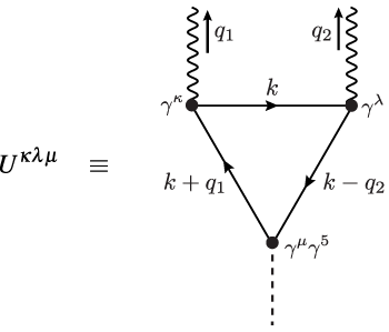
In quantum field theory, conservation laws result from analysis of the vertex functions. Analyzing the graphs in (8.117), one finds that the last graph, which contains a triangle-shaped fermionic closed loop, fails to satisfy the axial Ward identity and gives rise to the chiral anomaly. Let us now focus our attention on the triangle subgraph that couples AVV. As noted in the last lecture, there are other configurations such as AAA-triangle, squares, pentagons, etc. but to understand the basic mechanism of the chiral anomaly it suffices to consider the AVV graph. Since the photons are indistinguishable, there are two graphs that enter. They can be expressed in terms of two permutations of the diagram shown to the right.
The resulting Feynman diagrams can be expressed in terms of the three-tensor

where

with
 . The factor of
 arises from a sum over colored light quark
loops and is
arises from a sum over colored light quark
loops and is

where
 and
and
 .
.
Generally, the quantity
 is the Fourier transform of the AVV current
amplitude
is the Fourier transform of the AVV current
amplitude

The diagrams result from the perturbative expansion of this quantity
We can now check the various conservation laws
 and
and
 . Based on the last equation, current
conservation for the vector and axial-vector currents gives the following
conditions
. Based on the last equation, current
conservation for the vector and axial-vector currents gives the following
conditions

Looking at the first one, which expresses current conservation at one of the electromagnetic vertices, we find
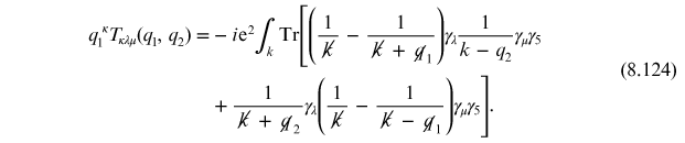
The integrals involving a single factor of photon momentum
 or
or
 vanish since the Levi-Civita tensor
associated with the trace
vanish since the Levi-Civita tensor
associated with the trace

requires contraction with two independent momenta in order to be non-vanishing. Defining

one finds

This integral linearly
divergent in the ultraviolet. If the integrals above were convergent, or diverged at
worst logarithmically, then we could shift the integration variables by
 in the first term and by
 in the second term and they would exactly
cancel. The linear divergence, however, means that this shift would appear in the upper
limit of the integration due to the need for regulation, and would break the symmetry
between the two terms. In order to carry out the shift more carefully, we Taylor
expand
in the second term and they would exactly
cancel. The linear divergence, however, means that this shift would appear in the upper
limit of the integration due to the need for regulation, and would break the symmetry
between the two terms. In order to carry out the shift more carefully, we Taylor
expand

to obtain

The omitted higher-order
terms in the Taylor series vanish when we remove the cutoff since, in the case at hand,
 and the integration measure contains a factor
of
and the integration measure contains a factor
of  . One can use Gauss' law to evaluate the
resulting integral, which gives (homework)
. One can use Gauss' law to evaluate the
resulting integral, which gives (homework)

where we have used
which gives

Similarly, one finds

and

This implies that current is not conserved and that electromagnetic gauge invariance is broken. Since gauge symmetry is special we can redefine the amplitude for the triangle graph by adding a polynomial in the external momentum, which can be be done without affecting the absorptive component of the amplitude. Thus, defining the physical decay amplitude via

we can enforce electromagnetic gauge invariance

at the expense of a non-vanishing axial divergence

and the axial current is no longer conserved. Using the last expression we have

Using
this maps to the condition

This is precisely the same form, we obtain based on more physical argumentation (8.105). If we were to repeat this exercise, without taking the fermion masses to zero in the beginning, we would have found instead

Exercise 8.11 Derive equation (8.119).
Exercise 8.12 Derive equation (8.123).
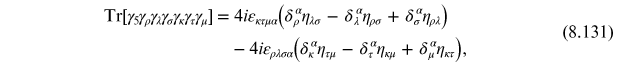
Exercise 8.13 Derive equation (8.130).
References
- [1]Dodd R K 1984 Solitons and Nonlinear Wave Equations (New York: Academic)
- [2]Kleinert H 1989 Gauge Fields in Condensed Matter (Singapore: World Scientific)
- [3]Deser S 1976 Phys. Lett. 64B 463–4
- [4]Huang K 1981 Quarks, Leptons and Gauge Fields (Singapore: World Scientific)
- [5]Weinberg S 1975 Phys. Rev. D11 3583–93
- [6]'t Hooft G 1976 Phys. Rev. Lett. 37 8–11
- [7]'t Hooft G 1976 Phys. Rev. D14 3432–50
- [8]Shifman M A, Vainshtein A I and Zakharov V I 1980 Nucl. Phys. B166 493–506
- [9]Baluni V 1979 Phys. Rev. D19 2227–30
- [10]Crewther R J, Di Vecchia P, Veneziano G and Witten E 1979 Phys. Lett. 88B [Erratum: Phys. Lett. 91B, (1980)] 123
- [11]Adler S L 1969 Phys. Rev. 177 2426–38
- [12]Bell J S and Jackiw R 1969 Nuovo Cim. A60 47–61
- [13]Bardeen W A 1969 Phys. Rev. 184 1848–57
- [14]Ananthanarayan B and Moussallam B 2002 J. High Energy Phys. 05 052
- [15]Goity J L, Bernstein A M and Holstein B R 2002 Phys. Rev. D66 076014
- [16]Kampf K and Moussallam B 2009 Phys. Rev. D79 076005
- [17]Landau L D 1981 Quantum Mechanics: Non-Relativistic Theory (Oxford: Butterworth-Heinemann)
- [18]Kharzeev D E, McLerran L D and Warringa H J 2008 Nucl. Phys. A803 227–53
- [19]Kharzeev D 2006 Phys. Lett. B633 260–4
- [20]Kharzeev D and Zhitnitsky A 2007 Nucl. Phys. A797 67–79
- [21]Kharzeev D E 2014 Prog. Part. Nucl. Phys. 75 133–51
- [22]Callan C G, Dashen R F and Gross D J 1978 Phys. Rev. D17 2717
- [23]'t Hooft G 1986 Phys. Rept. 142 357–87
- [24]Diakonov D 1996 Proc. Int. Sch. Phys. Fermi 130 (Preprint hep-ph/9602375) 397–432
- [25]Schäfer T and Shuryak E V 1998 Rev. Mod. Phys. 70 323–426
Footnotes
- 1
- 2
Since the ABJ result was obtained in the chiral limit (massless light quarks), it was not expected to be in full agreement with the data. Subsequent calculations using chiral perturbation theory have shown that, taking into account explicit chiral symmetry breaking, one obtains a lifetime, which is approximately 4% higher than the original ABJ calculation. See, for example, refs. [14–16].
- 3