


Abstract
The solar wind can directly interact with the lunar surface and provide an important source for surface space weathering and water generation. Here we study the solar wind implantation flux on the lunar surface with global Hall MHD simulations. The shielding effects of both the Earth's magnetosphere and lunar magnetic anomalies are considered. It is found that a large-scale lunar mini-magnetosphere can be caused by the solar wind interaction with the magnetic anomalies on the lunar far side, which causes a large shielding area on the surface. In addition, the Earth's magnetosphere brings a longitudinal variation in the implantation flux, with minimum fluxes at 0° longitude. With the integrated flux over a lunation, we find that there are some local cavities on the implantation flux map, which are colocated with both the magnetic anomalies and the lunar swirls. Further studies show that there is a south–north asymmetry in the implantation flux, which can be used to explain the lower water content observed in the southern hemisphere. Our results provide a global map of the solar wind implantation flux on the lunar surface and are useful for evaluating the large-scale effect of solar wind implantation and sputtering on the space weathering and the water or gas generation of the surface.
Export citation and abstract BibTeX RIS

Original content from this work may be used under the terms of the Creative Commons Attribution 4.0 licence. Any further distribution of this work must maintain attribution to the author(s) and the title of the work, journal citation and DOI.
1. Introduction
The Moon represents an airless body with no global magnetic field nor significant atmosphere, where solar wind can directly interact with the lunar surface. While a small part of the solar wind protons are reflected from the surface (0.1%–1% as H+—Saito et al. 2008; and 10%–20% as energetic neutral atoms, or ENAs—Wieser et al. 2009; Futaana et al. 2012), most solar wind particles are implanted into the surface, leaving a plasma cavity downstream from the Moon (Xie et al. 2012). These implanted solar wind particles can alter the physical and compositional properties of the lunar surface and result in a space-weathering process of the surface (Pieters & Noble 2016). Meanwhile, some lunar surface components, such as O, Si, Fe, and Ca, can be released from the surface by solar wind sputtering, providing an important source for the lunar exosphere (Wurz et al. 2007; Sarantos et al. 2012). In particular, the infrared absorption feature centered at 2.8 μm shows that the abundance of H2O/OH on the lunar surface has a diurnal variation, with higher concentrations near the terminator/polar regions (Sunshine et al. 2009; McCord et al. 2011; Li & Milliken 2017), suggesting that the solar wind implantation is the dominant source for the lunar water group species (H2O/OH).
Recent observations show that the Moon has a large number of local crustal magnetic fields, known as magnetic anomalies (Mitchell et al. 2008; Tsunakawa et al. 2015). Some strong magnetic anomalies can stand off or deflect the incoming solar wind and reduce the solar wind flux on the lunar surface. The Chandrayaan-1 spacecraft found that the lunar surface with magnetic anomalies has less backscattered ENAs (Wieser et al. 2010; Vorburger et al. 2013), implying that the surface was shielded by a lunar mini-magnetosphere (LMM). The LMM was also seen by the Chang'E-4 (CE-4) rover on the lunar surface, where the solar wind flux was reduced by about half by the LMM (Xie et al. 2021, 2022). Such a magnetic shielding can hinder the solar wind interaction with the lunar surface and bring some inhomogeneities to the surface properties. On the one hand, the lunar surface can be less space-weathered and a swirl may appear associated with the magnetic anomaly (Hood & Schubert 1980; Blewett et al. 2011; Glotch et al. 2015; Denevi et al. 2016). On the other hand, the surficial water content in the magnetic anomaly region can be smaller than the surrounding area (Li & Milliken 2017; Li & Garrick-Bethell 2019).
It is important to know the solar wind implantation flux on the lunar surface for both surface-weathering and water production studies. In simple terms, the implantation flux can be calculated as  , where Nsw, Vsw, and χ are the number density, velocity, and incidence angle of the solar wind, respectively. Previously, this term of the implantation flux was widely used to study the contribution of solar wind sputtering to the lunar exosphere (Wurz et al. 2007; Sarantos et al. 2012) and the migration of H-bearing species (OH, H2O, and H2) from the subsolar region to the polar region (Crider & Vondrak 2000; Tucker et al. 2019). In addition, a latitude-dependent space-weathering effect was observed by the Clementine spacecraft, consistent with the lower solar wind flux at higher-latitude regions (Hemingway et al. 2015). However, the Moon can receive lower solar wind flux when it is in the Earth's magnetosphere, which will bring a longitudinal variation in the implantation flux and cause an east–west difference in the spectrum of the crater wall, as seen by the SELENE spacecraft (Sim et al. 2017). Moreover, such a magnetospheric shielding can also affect the distribution of H-bearing species (Tucker et al. 2021).
The global features of the solar wind interaction with the Moon can be reproduced by either an MHD model (Xie et al. 2012) or a hybrid model (Holmstrom et al. 2012). Nevertheless, the interaction between the solar wind and magnetic anomalies has a scale smaller than the ion gyroradius or ion inertial length, in which the fluid assumption is invalid. A particle-in-cell (PIC) model can capture the most physics of interest. In particular, the effects of both the E × B drift and the ∇B drift on the formation of the LMM can be discussed by a PIC model (Deca et al. 2015). However, the PIC simulation is very costly and a 3D PIC simulation is limited to studying the solar wind interaction with a single magnetic anomaly, such as Reiner Gamma (Deca et al. 2018, 2020). A hybrid model is able to simulate the solar wind interaction with a global map of magnetic anomalies (Fatemi et al. 2014). However, the spatial resolution of a hybrid model is still restricted, which makes it not easy to include a high-order crustal magnetic field model or to obtain a high-resolution solar wind implantation flux on the surface (Kallio et al. 2019). A Hall MHD model is appropriate when the spatial scale is comparable to or smaller than the ion inertial length, due to the inclusion of the Hall term in the generalized Ohm's law (Toth et al. 2008). Moreover, a Hall MHD model has a low computational expense and a high spatial resolution, which make it easier to include a high-order crustal magnetic field model and obtain a high-resolution picture of the solar wind interaction with lunar magnetic anomalies. Previously, Harnett & Winglee (2003) first used a Hall MHD model to study the solar wind interaction with a lunar magnetic anomaly and found that the multipolar nature of the crustal field could increase the lateral extent of the interaction and help to form an LMM. Xie et al. (2015) developed a global Hall MHD model for the interaction between the solar wind and the Moon with a 178° spherical harmonic crustal field model, which could successfully capture the two continuous LMMs observed by the Chang'E-2 spacecraft. Recently, the model was improved with a 450° spherical harmonic crustal field model, and the simulation results could reproduce the partially shielded LMM as observed by the CE-4 rover (Xie et al. 2021).
In this paper, we try to study the global features of solar wind implantation flux on the lunar surface, with the model used in Xie et al. (2021). In particular, the shielding effects of both the Earth's magnetosphere and the lunar magnetic anomalies are considered. We will introduce some details about the model in Section 2 and examine the validity of the model by comparing the simulation results with the observations. The maps of the solar wind implantation flux at different lunar phases will be shown in Section 3, in which the long-term effects of the solar wind implantation associated with magnetic anomalies will be discussed. Finally, we will summarize this work in Section 4.
2. Model Description and Validation
We choose the Selenocentric Solar Ecliptic (SSE) coordinate system to describe the physical vectors, in which the X-axis points from the Moon's center to the Sun, the Z-axis is normal to the ecliptic plane, and the Y-axis completes the right-handed set of axes. The simulation domain is set to X = [−8, 2] RL , Y = Z = [−5, 5] RL , where RL = 1738 km is the lunar radius. The solar wind moves in the −X-direction as an inflow boundary, and the lunar surface is regarded as the inner boundary. The lunar body is treated as an insulated sphere for its low conductivity, and an absorbing or float boundary condition is applied at the inner boundary, which means that all the variables of the solar wind (both the plasma and the field) can pass the lunar surface freely. The lunar crustal fields are obtained by a 450° spherical harmonic model (Tsunakawa et al. 2015). A locally refined spherical grid is used, in which the smallest cell near the surface has a size of about 8 km in the radial direction and about 16 km in the horizontal direction. Such a cell is smaller than the wavelength of the 450° spherical harmonic model (about 24 km) and is refined enough to capture the spatial variation of the crustal magnetic fields. We choose a total variation diminishing scheme with second-order accuracy to solve the spatial discretization of the Hall MHD equations and a two-state local time-stepping method to solve the time discretization (Toth et al. 2008), and the numerical simulations are carried out by the Space Weather Modeling Framework (Toth et al. 2012).
To check the validity of the model, we carry out a global Hall MHD simulation for the joint LMM observation by the ARTEMIS spacecraft and the CE-4 rover during 01:00–08:00 UT on 2019 December 31 (Xie et al. 2022), when the ARTEMIS P2 spacecraft observed a significant shock in orbit and the CE-4 rover measured a reduced ENA flux on the lunar surface. The solar wind conditions are obtained by the ARTEMIS P1 spacecraft upstream from the shock, which have a number density of 21.95 cm−3, a temperature of 6.89 eV, a velocity of (−293.96, 12.35, −1.73) km s −1, and an interplanetary magnetic field of (2.30, 1.93, 5.83) nT. The subsolar point is approximately located at 125° east longitude and 0° latitude, and the CE-4 rover is located at (0.4284, 0.556 3, −0.7120) RL , with a solar zenith angle of about 65° during this period. As shown in Figure 1(a), the simulation produces a large-scale LMM that can been seen by both ARTEMIS P2 and CE-4. We extract the data along the trajectory of ARTEMIS P2 (the black dots in Figure 1(a)) and compare them with the observations. As shown in Figures 1(b)–(e), both the simulation and the observation show a similar shock structure around 02:15 UT, including jumps in the density and field strength, deceleration and deflection in the velocity, and rotations in the magnetic field. After entering the shock, both the density and the field strength keep decreasing. Moreover, the density and the field strength can be smaller than their undisturbed upstream values after 02:28 UT (Figures 1(b) and (c)), suggesting a plasma cavity inside the shock. To make sure whether the plasma cavity is related to the magnetotail of the LMM or the rarefaction region of the lunar wake, we carry out another simulation with the same solar wind parameters, but with no magnetic anomaly. As shown in Figures 1(b) and (c), the plasma cavity is emptier than the lunar wake. Consequently, we conclude that the reduced density and field are associated with the LMM's magnetotail.
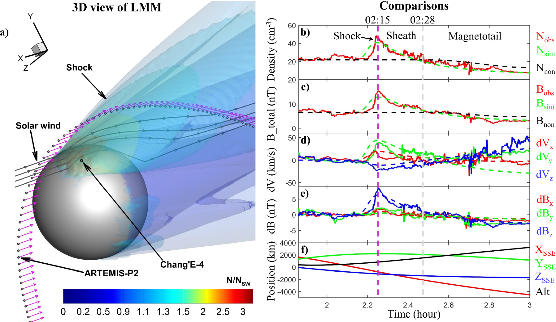
Figure 1. Comparison between the global Hall MHD simulation and the observation. (a) 3D view of the simulation results, where the central sphere represents the lunar body with color contours, to show the relative number density to the solar wind density (N/Nsw); the black dots show the trajectory of ARTEMIS P2 with magenta arrows, to indicate the velocity vectors extracted from the simulation results; the black circle on the lunar surface indicates the location of CE-4; and the gray lines show the streamlines of the solar wind. (b)–(e) Comparisons between the simulation results and the observations from ARTEMIS P2, in which the simulation results are shown as dashed lines, while the observation results are shown as solid lines: the lines with different colors indicate the results of different variables; the black dashed lines in (b) and (c) show the simulation results of the lunar wake with no crustal magnetic field; and the vertical magenta and gray dashed lines indicate the moments when the spacecraft encounters the shock and the magnetotail of the LMM, respectively. (f) Locations of ARTEMIS P2 in SSE coordinates, in which the red, green, and blue lines show the locations in the X-, Y-, and Z-directions, respectively, and the black line shows the altitude of ARTEMIS P2.
Download figure:
Standard image High-resolution imageAccording to the CE-4 observations, both the solar wind kinetic energy and the number flux have been reduced in this event, with a deceleration rate of 0.34 and a shielding efficiency of 0.67 (Xie et al. 2022), in which the deceleration rate is defined as 1-Ek
/Ek,sw and the shielding efficiency is defined as 1-ηsw, where Ek
and Ek,sw are the kinetic energies of deflected ions and the undisturbed solar wind, respectively, and ηsw is the penetrating efficiency. Here we extract the results of the number density (N) and velocity (V) from the global Hall MHD simulation and calculate the implanted number flux on the lunar surface via J = NVr
, where Vr
is the radial component of V. We use the normalized number flux defined as J/Jsw, where Jsw = Nsw
Vsw, to show the distribution of the implanted number flux on the lunar surface. As shown in Figures 2(a) and (b), a large area of lunar surface has been shielded from the solar wind, associated with the large-scale LMM shown in Figure 1(a). We define the penetrating efficiency as ηsw = J/Jsw,n, where  is the normal component of the solar wind flux at the position with a solar zenith angle of χ. As shown in Figure 2(c), we can find a large shielding area around CE-4 with ηsw < 1, and the ηsw near the CE-4 location is about 0.15. Meanwhile, there is a decrease in the ion kinetic energy due to the magnetic shielding, and the Ek
at the CE-4 location is about 57% of the Ek,sw as shown in Figure 2(d). Accordingly, we obtain a deceleration rate of 0.43 and a shielding efficiency of 0.85 from the simulation. These two values are both a little bit larger than the values measured by CE-4. The reason for such a difference may come from the absence of particle dynamics, such as ion gyromotion, in the Hall MHD model. In spite of this, the simulation results are still comparable to those of the observations. Combined with the comparison shown in Figure 1, we conclude that the global Hall MHD simulation can capture the main features of the LMM observed by ARTEMIS and CE-4. As a result, we think that the Hall MHD model is valid for simulating the global solar wind interaction with lunar magnetic anomalies and applicable to studying the solar wind implantation flux on the lunar surface.
is the normal component of the solar wind flux at the position with a solar zenith angle of χ. As shown in Figure 2(c), we can find a large shielding area around CE-4 with ηsw < 1, and the ηsw near the CE-4 location is about 0.15. Meanwhile, there is a decrease in the ion kinetic energy due to the magnetic shielding, and the Ek
at the CE-4 location is about 57% of the Ek,sw as shown in Figure 2(d). Accordingly, we obtain a deceleration rate of 0.43 and a shielding efficiency of 0.85 from the simulation. These two values are both a little bit larger than the values measured by CE-4. The reason for such a difference may come from the absence of particle dynamics, such as ion gyromotion, in the Hall MHD model. In spite of this, the simulation results are still comparable to those of the observations. Combined with the comparison shown in Figure 1, we conclude that the global Hall MHD simulation can capture the main features of the LMM observed by ARTEMIS and CE-4. As a result, we think that the Hall MHD model is valid for simulating the global solar wind interaction with lunar magnetic anomalies and applicable to studying the solar wind implantation flux on the lunar surface.

Figure 2. (a)–(d) The simulation results of the magnetic field (B), the normalized number flux (J/Jsw), the penetrating efficiency (ηsw), and the normalized kinetic energy (Ek /Ek,sw) of the solar wind on the lunar surface, respectively. The white dotted lines indicate the terminators during this period, and the solid dot marks out the location of CE-4.
Download figure:
Standard image High-resolution image3. Solar Wind Implantation Flux Map
In reality, the Moon spends about one-quarter of its orbit in the Earth's magnetosphere. Additionally, the solar wind conditions can vary in time. For simplicity, here we consider a steady solar wind condition, with a number density of 5 cm−3, a temperature of 10 eV, a velocity of [−400, 0, 0] km s−1, and a magnetic field of [−5, 5, 0] nT in the Geocentric Solar Ecliptic (GSE) coordinate system. The global structure of the Earth's magnetosphere is obtained by the PPMLR-MHD model (Hu et al. 2007; Wang et al. 2013), which is an advanced global model with high-order spatial accuracy and low numerical dissipation. As shown in Figure 3, we neglect the tilt angle of the Earth and assume that the lunar orbital plane coincides with the ecliptic plane. In this way, the Moon moves in the GSE XY-plane with a distance of about 60 RE to the Earth. We use phase angles in the GSE coordinate system (ϕGSE) to indicate the different locations of the Moon around the Earth. ϕGSE = 0° means that the Moon is in the upstream solar wind and ϕGSE = 180° means that the Moon is in the Earth's magnetotail. We choose eight typical phase angles with an increment of 45° (the circled dots in Figure 3) to show the variation of the solar wind implantation flux map during different lunar phases. In addition, we divide the whole lunar orbit into 72 segments with intervals of 5° (the black dots in Figure 3) to obtain the integrated implantation flux over one lunar orbit (or lunation).

Figure 3. Different locations of the Moon during its orbit around the Earth. The color contours show the number densities of the Earth's magnetosphere obtained from the global PPMLR-MHD simulation. The black dots show the different lunar locations in the GSE XY-plane with intervals of 5°. The circled dots indicate the locations with intervals of 45°, whose implantation flux maps are shown in this work.
Download figure:
Standard image High-resolution imageWe first extract the plasma parameters at a specific lunar location from the results of Earth's global PPMLR-MHD simulation, which are then used as the input parameters for the lunar global Hall MHD simulation. With the number density and velocity results from the global Hall MHD simulation, we can calculate the implanted number flux on the lunar surface. As shown in Figure 4(a), the normalized number flux basically shows a circular shape with the maximum flux at the subsolar point, consistent with a cosine function of the solar wind incidence angle. However, the circular shape can be interrupted by the magnetic anomalies due to the magnetic shielding effect. Furthermore, there are some enhanced fluxes just outside the shielded regions (especially when ϕGSE = 45° and ϕGSE = 270°), associated with the deflection and compression of the solar wind in these regions. Similar enhanced flux regions were also seen in the ENA observations (Wieser et al. 2010; Xie et al. 2021). Apart from the shielding of lunar magnetic anomalies, there is also a shielding of the Earth's magnetosphere, which leads to a very low implanted flux when ϕGSE = 180°. In addition, the flux can be enhanced overall when the Moon is in the Earth's magnetosheath (ϕGSE = 135° and ϕGSE = 225°); in particular, the implantation flux around 0° longitude is enhanced.

Figure 4. (a) The maps of implanted number flux at different phase angles, in which the number fluxes are normalized by the solar wind number flux. (b) The maps of implanted energy flux at different phase angles, in which the energy fluxes are normalized by the solar wind energy flux.
Download figure:
Standard image High-resolution imagePreviously, Deca et al. (2018) found that the albedo pattern of the Reiner Gamma swirl was better correlated with the energy flux, rather than the number flux, suggesting that the space-weathering process was mainly controlled by the energy flux of the solar wind. In fact, the effect of solar wind implantation on the space weathering and water generation is quite dependent on the penetrating depth of the solar wind in the regolith. Since the penetrating depth is determined by the solar wind energy, we can find a better correlation between the space weathering and the energy flux. Nevertheless, apart from the solar wind energy, both the experiments (Overbury et al. 1980) and the numerical simulations (Szabo et al. 2022) have shown that the incidence angle is also important to determining the penetrating depth. As a result, here we choose the normal component of the solar wind kinetic energy to calculate the energy flux, which is defined as  . Here we find that the solar wind protons are only partially shielded by the magnetic anomaly, especially for weak magnetic anomalies. As a result, the number flux reduction in the crustal field region is not so significant due to the solar wind penetration. Meanwhile, there is a deceleration and deflection along with the penetration, leading to a reduced energy flux in the normal direction. Consequently, the energy flux is more sensitive to the magnetic anomalies, and we can find more cavities in the map of energy flux (Figure 4(b)). In addition, we fail to see enhancement regions surrounding the cavities in the energy flux map even when ϕGSE = 45° and ϕGSE = 270°, implying that the solar wind protons have been decelerated during the deflection around the magnetic anomaly.
To investigate the long-term effect of solar wind implantation and relate it to the space weathering of the lunar surface, we calculate the integrated implantation flux over one lunation. We divide the lunar orbit into 72 intervals and calculate the normalized implantation flux (number flux or energy flux) for each interval with the global Hall MHD model. We add all of the normalized fluxes together and divide the sum by 72 to obtain the average flux per lunation. Such an average flux can be used to evaluate the long-term effect of solar wind implantation. As shown in Figure 5, both the average number flux and the average energy flux are decreasing with an increasing latitude, associated with the dependence on solar wind incidence angles. Additionally, these fluxes show a longitudinal variation with a minimum flux at 0° longitude, caused by the shielding of Earth's magnetosphere. Nevertheless, the flux at 0° longitude is still comparable to that at 180° longitude (the ratio is larger than 50%), caused by the flux enhancement in the Earth's magnetosheath. In addition, there are many local flux cavities associated with the magnetic anomalies. These cavities are colocated with most lunar swirls found by Blewett et al. (2011) and Denevi et al. (2016), especially for the cavities in the energy flux map (Figure 5(c)). It should be noted that our results can only reflect the large-scale feature (the shielding effect on the scale of the ion inertial length) of the implantation flux near the swirls, but cannot reproduce the fine structure, such as the dark lanes, inside the swirl, since the fine structure has a spatial scale of about 1 km, which is about 1 order magnitude smaller the grid size used in our simulation. Moreover, there are also some regions that have magnetic anomalies and flux cavities, but are without a swirl, such as the region to the north of the NW of Apollo region. This implies that the swirl formation is also affected by some other factors, such as the exposure age and the mineral composition. In general, our results provide a global map of the solar wind implantation flux on the lunar surface, with the shielding effect of lunar magnetic anomalies.
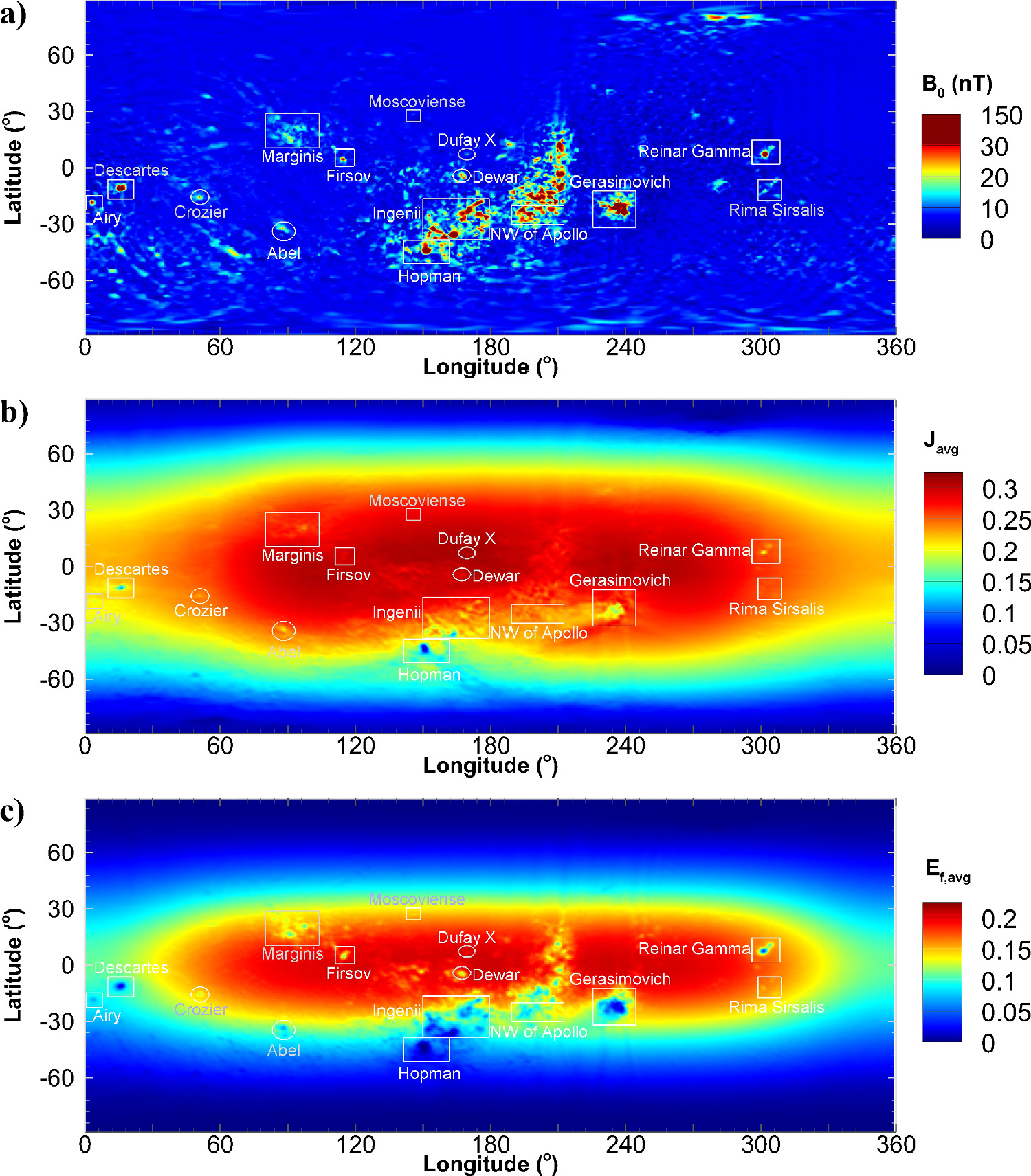
Figure 5. (a) The map of the magnetic field strength on the lunar surface, obtained from the 450° spherical harmonic model (Tsunakawa et al. 2015). (b) The map of the average number flux (Javg) over one lunation. (c) The map of the average energy flux (Ef,avg) over one lunation. The rectangles indicate the locations of the lunar swirls examined by Blewett et al. (2011) and the circles indicate the locations of the other lunar swirls found by Denevi et al. (2016), accompanied by the names of nearby magnetic anomalies.
Download figure:
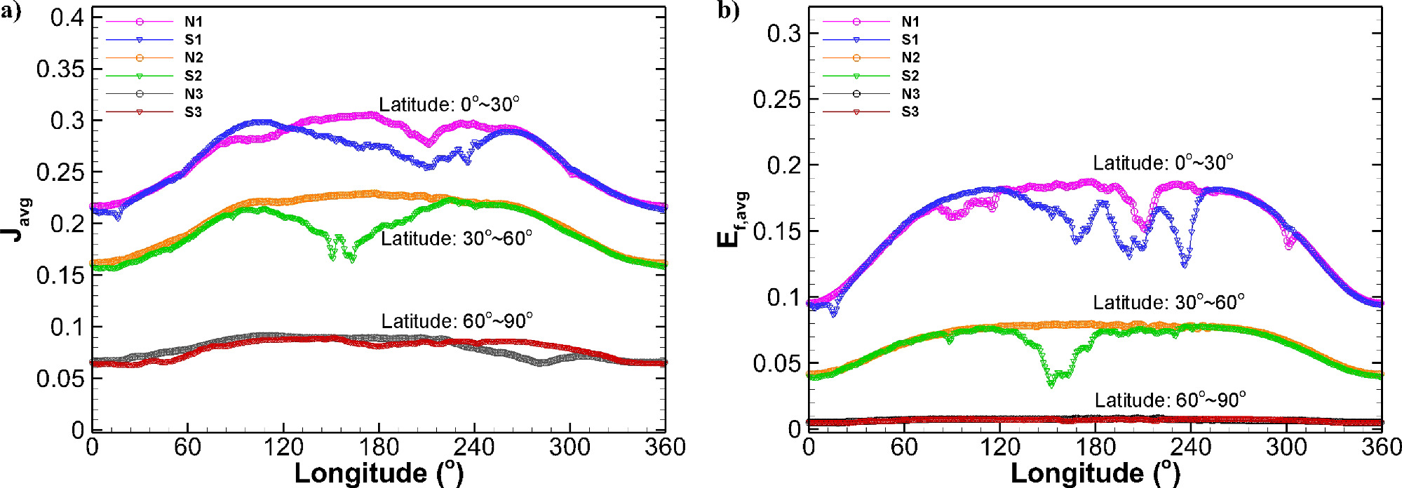
Standard image High-resolution imageSome cavities, such as those located at the Hopman, Ingenii, NW of Apollo, and Gerasimovich magnetic anomalies, can have a width as large as 1000 km, which may bring some global influences on the solar wind–Moon interaction. We calculate the average fluxes in three different latitude ranges, known as the low-latitude range (0°–30°), the mid-latitude range (30°–60°), and the high-latitude range (60°–90°), respectively. As shown in Figure 6, the implantation fluxes show clear south–north differences at the low and middle latitudes, but the difference at high latitudes is not clear. In particular, the maximum difference occurs near 150° longitude in the mid-latitude range, where the number flux (the energy flux) in the southern hemisphere is about 30% (50%) lower than that in the northern hemisphere. As known from Figure 5, such a difference is mainly caused by the Hopman magnetic anomaly. In addition, there is a south–north difference of about 10% between 120° and 250° longitude for the low-latitude range, which is associated with the Ingenii, NW of Apollo, and Gerasimovich magnetic anomalies. Previously, both the neutron spectra (Feldman et al. 1998) and M3 data (Li & Milliken 2017) showed that the water content in the southern hemisphere was generally lower than that in the northern hemisphere. According to the Monte Carlo simulation (Crider & Vondrak 2000), the water molecules from the solar wind implantation can migrate from the subpolar point to the pole region, and the low and middle latitudes of the northern (southern) hemisphere are the main source for the water in each hemisphere. Here we find a wide area of reduced implantation flux in the southern hemisphere at both the low and middle latitudes, which corresponds to a lower water production rate in these areas. That may be the reason for the lower water content observed in the southern hemisphere. It should be noted that the water distribution in the polar region is more complicated than we thought. Larger areas of ice exposure have been found in the southern pole, which can be caused by either the more permanently shaded area (Li et al. 2018) or the magnetically reduced solar wind sputtering (Hood et al. 2022) in the southern pole region.
Figure 6. Comparisons of the implantation fluxes in the southern hemisphere and the northern hemisphere. (a) and (b) Comparisons of the average number flux and the average energy flux, respectively. The magenta, yellow, and gray dots indicate the average fluxes in the northern hemisphere, with latitude ranges of 0°–30°, 30°–60°, and 60°–90°, respectively. The blue, green, and red dots indicate the average fluxes in the southern hemisphere, with latitude ranges of 0°–30°, 30°–60°, and 60°–90°, respectively.
Download figure:
Standard image High-resolution image
4. Conclusions and Discussions
We study the global features of the solar wind interaction with lunar magnetic anomalies with a global Hall MHD model and calculate the solar wind implantation flux on the lunar surface. It is found that there is a large shielding area with a lower implantation flux on the lunar far side. In addition, the implantation flux varies with different lunar locations during its orbit around the Earth, with the maximum flux in the magnetosheath and the minimum flux in the magnetotail. We use the integrated flux over a lunation to investigate the long-term effect of solar wind implantation and find that the integrated flux can decrease with an increasing latitude and with a longitude approaching 0°. Additionally, there are some local cavities in the flux map, associated with the shielding effect of the lunar magnetic anomalies. These flux cavities gather in the southern hemisphere and bring a south–north asymmetry in the implantation flux, especially at the low and middle latitudes.
It is interesting to find that the flux cavities are approximately colocated with the locations of lunar swirls. In addition, the south–north asymmetry in the implantation flux can be used to explain the lower water content observed in the southern hemisphere. This suggests that our results have captured the large-scale shielding feature of the solar wind interaction with lunar magnetic anomalies, and the implantation flux can be used as an input parameter for lunar surface-weathering and water generation studies. Similarly, we can also use the implantation flux to study the contribution of solar wind sputtering to the lunar exosphere. Next, a Monte Carlo model is needed to study the shielding effect of magnetic anomalies on the generation and migration of water molecules and other exospheric species.
It should be noted that the actual processes of space weathering and water formation can be more complicated than we thought. Apart from the solar wind implantation, both the chemical composition and the exposure age of the lunar regolith can affect the space weathering. In addition, the solar wind can provide either a source for the lunar water through implantation (especially at low and middle latitudes) or a loss for the lunar water through sputtering, especially in the shadowed polar region (Farrell et al. 2019). Furthermore, both the earth wind (Wang et al. 2021) and the high-energy electrons from the plasma sheet of the Earth's magnetotail (Li et al. 2023) may contribute to the lunar water, and the ice exposure area in the polar region is quite dependent on the area of permanently shaded craters (Li et al. 2018). All of these factors are not considered in our model, which could bring some deviations between the simulated implantation flux and the spectral feature or water content of the lunar surface, and should be carefully treated in future studies. In summary, we provide a global implantation flux map of solar wind protons on the lunar surface, which can help people to understand the large-scale features of solar wind implantation on the lunar surface and has general implications for studying the space weathering, water production, and sputtering of the surface.
Acknowledgments
This work was supported by the National Natural Science Foundation of China (grant No. 42174216) and by the National Key R&D Program of China (grant No. 2020YFE0202100). This work was also supported by the Pandeng Program of the National Space Science Center, Chinese Academy of Sciences. L.X. was supported by the Youth Innovation Promotion Association of the Chinese Academy of Sciences. We acknowledge the CSEM team at the University of Michigan for the use of the SWMF code.