


Abstract
On 2022 March 4, the object known as WE0913A crashed into the Moon after several close flybys of the Earth and the Moon in the previous three months. Leading up to impact, the identity of the lunar impactor was up for debate, with two possibilities: the Falcon 9 from the DSCOVR mission or the Long March 3C from the Chang'e 5-T1 mission. In this paper, we present a trajectory and spectroscopic analysis using ground-based telescope observations to show conclusively that WE0913A is the Long March 3C rocket body (R/B) from the Chang'e 5-T1 mission. Analysis of photometric light curves collected before impact give a spin period of 185.221 ± 6.540 s before the first close Earth flyby on 2022 January 20 and a period of 177.754 ± 0.779 s, both at a 1σ confidence level, before the second close Earth flyby on 2022 February 8. Using Markov Chain Monte Carlo sampling and a predictive light curve simulation based on an anisotropic Phong reflection model, we estimate both physical and dynamical properties of the Chang'e 5-T1 R/B at the start of an observation epoch. The results from the Bayesian analysis imply that there may have been additional mass on the front of the rocket body. Using our predicted impact location, the Lunar Reconnaissance Orbiter was able to image the crater site approximately 7.5 km from the prediction. Comparing the pre- and post-impact images of the location shows two distinct craters that were made, supporting the hypothesis that there was additional mass on the rocket body.
Export citation and abstract BibTeX RIS

Original content from this work may be used under the terms of the Creative Commons Attribution 4.0 licence. Any further distribution of this work must maintain attribution to the author(s) and the title of the work, journal citation and DOI.
1. Introduction
On 2015 March 14, the Catalina Sky Survey (Christensen et al. 2018), which scans the sky for near-Earth objects, discovered a new object and provisionally named it WE0913A. This object was placed on the Near-Earth Object Confirmation page 7 of the Minor Planet Center. Subsequent observations showed that the object was in a geocentric orbit rather than heliocentric, suggesting it could be space junk. Furthermore, additional observations showed that the object had a lunar flyby on 2015 February 13. On 2015 February 11, NASA had launched the Deep Space Climate Observatory (DSCOVR) spacecraft toward the Earth–Sun L1 point on a Falcon 9 rocket from Cape Canaveral, Florida. Consequently, WE0913A was initially linked to the Falcon 9 rocket body (R/B; (NORAD ID 40391, COSPAR ID 2015-007B) that was used for the launch of the DSCOVR mission. This object was observed over the course of the next 6 yr and in late 2021 it became apparent that the object would impact the Moon in 2022 March, after close approaches with the Earth and Moon over the next three months.
On 2022 February 12, Jon Giorgini at the Jet Propulsion Laboratory (JPL) realized that WE0913A was unlikely to be the DSCOVR Falcon 9 R/B, as JPL Horizons ephemeris for DSCOVR did not show it being particularly close to the Moon after its launch in 2015. The original assumption that this was the DSCOVR R/B was more circumstantial than conclusive, and thus further investigation was required. Propagating the orbit of WE0913A backward past its lunar encounter in 2015 February gave another lunar encounter on 2014 October 28; and before that, the object looked to be on a typical lunar transfer orbit from the Earth. This timeline coincided with the launch of the Chinese Chang'e 5-T1 mission to the Moon on 2014 October 23. This led us to believe that the object that would impact the Moon on 2022 March 4 was likely the Long March 3C R/B (NORAD ID 40284, COSPAR ID 2014-065B) from the Chang'e 5-T1 mission. Adding to the confusion, after this realization, the Chinese Ministry of Foreign Affairs issued a press release on 2022 February 21 saying that the object impacting the Moon was not the Long March 3C upper stage from the Change 5 mission (Wenbin 2022).
In this paper, we present our characterization efforts using both astrometric and photometric data of WE0913A in order to provide insight into some dynamical and physical properties of the object that impacted the Moon on 2022 March 4. Using the astrometric data, an overview of our efforts to predict the impact location is also given. Additionally, we present telescopic visible-wavelength spectroscopy of the object in question and compare it to spectra collected of other Falcon 9 and Long March 3C rocket bodies in Earth orbit to show the spectral characteristics of each.
2. Observations and Data Reduction
The data products used directly in this research are the time history of reduced photometric brightness measurements (light curves) taken from imagery data acquired with each telescope. Astrometric position measurements are only used indirectly, being needed for orbit determination to allow for later trajectory propagation to support the reflective dynamics model (see Sections 6.1.2 and 6.1.3). All the imagery data used were collected from two telescopes located in Arizona, USA. Some basic information for each of the sensors can be found in Table 1.
Table 1. Relevant Parameters for the Sensors Used to Collect Data of the Chang'e 5-T1 R/B
| Name | Location | Aperture (m) | FOV (arcmin) | Pixel Size (as px−1) |
|---|---|---|---|---|
| Leo-20 | Arizona, USA | 0.52 | 81 × 81 | 2.4 |
| RAPTORS I | Arizona, USA | 0.61 | 16 × 16 | 0.95 |
Note. FOV stands for Field of View.
Download table as: ASCIITypeset image
All observations from Leo-20 were taken with an open/clear filter, and those from RAPTORS I were taken using the Sloan Digital Sky Survey g' and r' photometric filters with band passes (>50% transmission) of 401–550 nm and 555–695 nm, respectively. Visible spectra (450–950 nm) from RAPTORS I were taken with a 30 line mm−1 transmission diffraction grating installed in the light path, resulting in a 14.6 nm px−1 (R ∼ 30 at 450 nm) spectral resolution. Further details about the grating's throughput in each order and the process for determining the spectral resolution can be found in Battle et al. (2022, 2023). The observation geometry, dates, and number of images taken can be found in Table 2.
Table 2. Summary of Observation Epochs and Geometry for the Collected Data
| Name | Date (UTC) | Range (km) | V Mag (Pred.) | Phase Angle (°) | No. of Obs. |
|---|---|---|---|---|---|
| Leo-20 | 2022/01/20 | 169,000 | 15.3 | 91.4 | 400 |
| 2022/02/08 | 144,000 | 15.2 | 102.5 | 300 | |
| RAPTORS I | 2022/02/08 | 144,000 | 15.2 | 102.5 | 211 |
Download table as: ASCIITypeset image
The reduction and analysis of the telescope data are accomplished by first calibrating all images with dark, bias, and flat-field frames in order to reduce the amount of errant noise and vignetting in the images caused by the sensor system. Once the images are calibrated, the plate solution is calculated using the GAIA Data Release 2 star catalog (Gaia Collaboration 2018) and open-source software package Scamp (Bertin 2006). After a successful plate solution is found, the centroid and signal (flux) from the desired target (WE0913A) may be extracted via aperture photometry, accomplished here with the open-source software Source-Extractor (Bertin & Arnouts 1996). Reported observations are flux calibrated with up to a first-order correction calculated from solar analog stars across all the frames in a data set. Solar analog stars are selected based on the criteria given in Andrae et al. (2018).
Spectra are extracted from RAPTORS I images by summing the flux in each column along the spectrum. Wavelength is determined using the distance (in number of columns only) from the centroid multiplied by the grating resolution. The flux in each wavelength unit is divided by the flux in the same wavelength unit for a solar analog spectrum to obtain a reflectance value. The reflectance spectrum is then normalized to unity at 700 nm.
3. WE0913A Trajectory Analysis
The Chang'e 5-T1 mission launched on 2014 October 23 at 18:00 UTC from the Xichang Satellite Launch Center, and according to the Long March 3C user manual (Cen et al. 2011), during a "typical flight sequence" the second third-stage powered flight (which takes the payload from an Earth parking orbit onto its translunar trajectory) occurs between 1323.2 and 1494.9 s post liftoff. Preceding this burn, the rocket/payload combination is in a "coast phase" for roughly 11 minutes. This point when the rocket/payload combination leaves its Earth parking orbit marks the periapsis of its lunar transfer orbit.
Using observations collected in 2015 March, when WE0913A was first observed by the Catalina Sky Survey, we can fit an orbit and propagate the results backward in time to observe the history of the trajectory of the object. A plot of the trajectory of WE0913A is given in Figure 1.

Figure 1. Example of the WE0913A orbit (black curve) from 2015 March 15 propagated backward until it hits its perigee on 2014 October 23. Orbits are shown in the geocentric MEME J2000 equatorial reference frame. The Moon's orbit (gray curve) and Earth's location (black dot) are included for reference. The rocket body had close encounters with the moon on both 2015 February 13 and 2014 October 28.
Download figure:
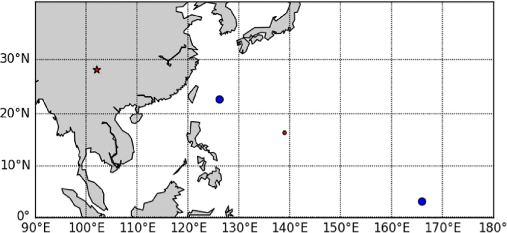
Standard image High-resolution imageIn Figure 2, we show a short ground track of the backward propagation up to perigee (denoted by a dot). The Xichang launch facility is also shown for reference (marked as a star). The time of perigee in Figures 1 and 2 should correspond with the time window between coast and translunar orbit injection that we described above, and we find that indeed it does. By following the description in the Long March 3C user manual, this phase should have occurred between 18:22:03.2 and 18:24:54.9 UTC on 2014 October 23. The results of our backward propagation put this perigee at 18:24:34.3 UTC. Moreover, the Long March 3C user manual lists the expected sublatitudes and sublongitudes for the launch vehicle during its initial phases of flight. Figure 3 shows the two launch phases as large dots and our derived perigee as a small dot. Again, the launch facility is included as a star for reference. As can be seen in this figure, the perigee falls squarely between these two launch phases, both geographically and in time.

Figure 2. Ground track of WE0913A (red curve) showing the orbit propagated backward to perigee (red dot) on 2014 October 23 at 18:24:34.3 UTC (24 minutes after Chang'e 5-T1 launch). Only a short time near perigee is shown for simplicity. The Xichang Satellite Launch Center, from which the Chang'e 5-T1 mission was launched, is shown as a red star.
Download figure:
Standard image High-resolution image
Figure 3. Zoomed-in view of the WE0913A calculated perigee (red dot) with the context of the coast and final burn stages of launch (large blue dots). The Chang'e 5-T1 R/B translunar trajectory should have a perigee between these two points, and we see that this is the case. The time window between the two launch phases is T + 22.053 minutes and T + 24.915 minutes and our calculated perigee is at T + 24.572 minutes. The Xichang Satellite Launch Center is again shown as a red star.
Download figure:
Standard image High-resolution imageThe mean residual in our orbit determination from the observations of WE0913A used to recreate this trajectory is 0 3. In this model, we estimate parameters corresponding to solar radiation pressure (SRP), which must be considered for this length of propagation. For instance, without taking into account SRP, the time of perigee for this object is delayed to 20:55:30.8 UTC on 2014 October 23. A difference of 2.5 hr and a perigee slightly off-track from the launch path! However, the SRP parameters for a tumbling rocket body can be extremely hard to estimate and are, in fact, changing in time. As such, the parameters used represent a mean fit.
Based on this analysis, we show that the trajectory of WE0913A matches the nominal mission plan published in the Long March 3C user manual (Cen et al. 2011). Additionally, the WE0913A trajectory strongly indicates a launch from the Xichang Satellite Launch Center on 2014 October 23 at approximately 1800 UTC. As such, we may conclude that this object is likely to be the Long March 3C R/B (NORAD ID 40284, COSPAR ID 2014-065B) that launched the Chang'e 5-T1 mission.
4. Spectral Analysis
Spectroscopy has been shown to be a useful tool to identify space objects in Earth orbit based on their reflectance properties in the visible wavelengths (0.4–1.0 μm; Battle et al. 2023). Building upon the trajectory analysis results, we have spectral observations that favor the conclusion that the observed object was indeed the Chang'e 5-T1 R/B instead of the Falcon 9 R/B from the DSCOVR mission. In order to support this conclusion, we needed to observe comparison objects that had been launched at a similar time as the Chang'e 5-T1 R/B so that the materials used and any alterations from space aging would be similar (Jorgensen et al. 2001). Observations were taken of a Falcon 9 R/B (NORAD ID 40108, COSPAR ID 2014-046B) launched in 2014 August and a Long March 3C R/B (NORAD ID 43875, COSPAR ID 2018-110B) launched in 2018 December. These will be used to compare to the targets: the Falcon 9 R/B (NORAD ID 40391, COSPAR 2015-007B) used to launch the DSCOVR mission in 2015 February and the Long March 3C R/B (NORAD ID 40284, COSPAR ID 2014-065B) used to launch the Chang'e 5-T1 in 2014 October.
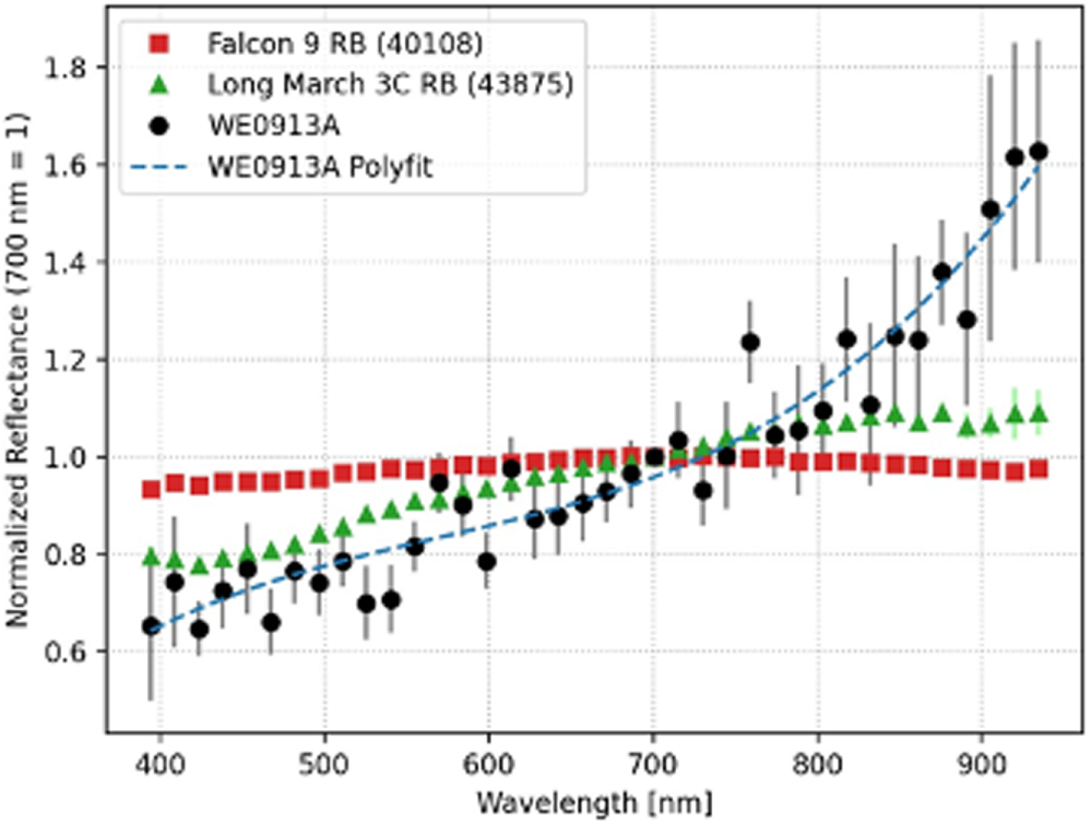
Figure 4 shows the collected spectrum of the lunar impactor (WE0913A) with spectra of the comparison objects and error bars representing the standard deviation of the reflectance measured across multiple images taken during observations. Since the WE0913A object was very faint for the RAPTORS I telescope (V mag 15.2) during the observations, the resulting low-resolution spectrum is noisy, so there is also included a plot of a third-order polynomial fit to the data for reference.

Figure 4. Normalized reflectance spectra from RAPTORS I showing a comparison between a Falcon 9 R/B (squares), a Long March 3C R/B (triangles), and the lunar impactor (dots). A third-order polynomial fit to the WE0913A data is provided as a reference. It is clear from the figure that the lunar impactor is a much closer spectral match to the Long March 3C R/B than the Falcon 9 R/B.
Download figure:
Standard image High-resolution imageThe spectrum of the Falcon 9 R/B (denoted by squares in Figure 4) is spectrally flat, reflecting blue (∼400 nm) and red (∼900 nm) light almost equally. The spectra for both the known Long March 3C R/B (triangles) and the lunar impactor (dots) are red-sloped, reflecting more red light than blue light. Although spectral slope is not necessarily diagnostic of what material or object is being observed, we can use these results to say which of the comparison objects the lunar impactor more closely matches. Using the third-order polynomial as expected values, we can use a Chi-squared measurement to quantify the degree to which the observed Falcon 9 and Long March 3C data match those of the lunar impactor. The Chi-squared value for the Long March 3C R/B (0.83) is lower (better match) than that of the Falcon 9 R/B (2.02), indicating that the Long March 3C R/B spectrum is a better match to the spectrum of the lunar impactor, further supporting the hypothesis that the lunar impactor was indeed the Long March 3C upper stage that launched the Chang'e 5-T1 mission. We will refer to WE0913A in the subsequent sections as the Chang'e 5-T1 R/B for clarity and conciseness.
Since all spectra involved in this analysis are relatively featureless, it is worth discussing potential causes of the difference in the spectral slopes seen in Figure 4 to better understand the implications for the object's origin. Potential explanations for the differences between these spectra include phase angle, space aging, and compositional differences (Pearce et al. 2020; Battle et al. 2023). Comparison objects were chosen that were launched at a similar time as the proposed origins of WE0913A so that the space aging impacts potentially would be similar and could largely be ignored. It is possible that WE0913A received higher amounts of radiation in deep space, and thus more space aging, compared to the comparison R/B that remained in low-Earth orbit (Reitz 2008; Restier-Verlet et al. 2021). Phase angle effects are harder to address, since there is no singular library of space-aged spacecraft material spectra at multiple phase angles to help address how phase angle effects manifest for different materials.
Additionally, we do not know the composition of the comparison R/Bs, which makes all comparisons more difficult. The major components of these R/B spectra, however, will typically include a white thermal control paint used on the exterior of the fuselage and the metal used for the engines. The composition of the thermal control material (TCM) used and its resistance to space aging may vary drastically between the Falcon 9 R/B and the Long March 3C R/B. Some white TCMs tend to yellow as they space age, while others are resistant to the changes and maintain a white appearance (Dever 1991; Bengtson et al. 2018; Goto et al. 2021). Although the exact paint is not known, it is plausible that the paint used on the Long March 3C R/B tends to yellow with exposure to the space environment, whereas the paint used on the Falcon 9 does not. This would create the observed difference in spectra between the two objects, despite similar times on orbit.
5. Photometric Analysis
Light curve inversion is a topic that has been extensively studied as it applies to asteroids and other natural bodies (Kaasalainen et al. 2001; Kaasalainen & Torppa 2001; Muinonen et al. 2020), the limitations of which, and general ill-posed nature of the problem, are well understood (Calef et al. 2006; Hinks et al. 2013); however, useful information can still be learned from even ill-posed inverse problems. These techniques have also been no less frequently applied toward artificial objects (Linares et al. 2013, 2014, 2020; Linares & Crassidis 2018). The focus has, however, almost exclusively been for characterization of shape or object type. There have been few attempts in the literature to apply these methods to a (partially) known object to assess the performance of a model-based approach with a comparison to real data. One such example is by Campbell et al. (2022), where they use this technique to look at cislunar object 2020 SO and recover several dynamical and physical properties. Originally discovered by Pan-STARRS1 and thought to be a natural object, it was later shown that 2020 SO was actually the Centaur upper stage from the Surveyor 2 mission. Another example (Santoni et al. 2013) also looks at recovering properties other than shape, but there are some clerical errors in the material characteristics and thus only diffuse reflection is considered, which is not sufficient for human-made objects with highly specular components. Moreover, the techniques used are shape-specific and significant rotational assumptions are made, so the methods are not applicable in general.
The photometric measurements taken on 2022 January 20 and February 8 show a strong apparent periodicity in the light curves of the Chang'e 5-T1 R/B that implies the object is neither actively stabilized nor tumbling (in the complex sense), but rather uniformly rotating (typically) about either its major or minor principal axes of inertia. It is also typical for objects rotating in this manner to then have a precession of this rotational axis about the body's angular momentum vector (Benson et al. 2017). To quantify this observed periodicity, we performed a four-parameter Fourier fit with least squares minimization to the light curves taken just before each of two sequential close Earth flybys. The results of these minimizations are in Figures 5(a) and (b).

Figure 5. Light curves of Chang'e 5-T1 R/B from before each of two sequential close Earth flybys taken from the same observatory. The light curves have been period wrapped by fitting a four-parameter Fourier series to the data via least squares minimization. As can be seen by the fitted period in each plot, the observed rotation rate of Chang'e 5-T1 changed substantially between the two flybys.
Download figure:
Standard image High-resolution imageFigures 5(a) and (b) show that the period of the light curve changes between the two observing epochs, indicating a likely change in the rotational period of the Chang'e 5-T1 R/B. While the period of the light curve just before the second Earth flyby is within the 2σ bounds of the first set of data, the reverse is not true, indicating that this is likely a real change in the rocket body's rotational rate. A high-fidelity attitude simulation and analysis may be able to lend insight into the impact of the first Earth flyby on the Chang'e 5-T1 R/B rotational period, but this is outside the scope of this work.
Using a predictive light curve model and Markov Chain Monte Carlo (MCMC) sampling-based inversion using astrometric and photometric data collected of the Chang'e 5-T1 R/B during both of its final close approaches with the Earth before impacting the Moon, we recover likely distributions for spin state and reflective properties. We estimate nine parameters: primary body axis orientation (2), angular velocity vector (3), diffusive/specular reflectivity parameters (2), and surface anisotropic/roughness parameters (2).
6. Bayesian Inversion Methodology
Bayesian inversion relies heavily on a statistical forward model that can map arbitrary samples in your chosen parameter space to realistic samples in the desired observation space. It is important to strike a good compromise between model fidelity and computational requirements for said model, since there are harsh diminishing returns for increased fidelity with ill-posed inverse problems.
In this research, our forward model takes as input an arbitrary set of the nine parameters we want to estimate: primary body axis orientation (2), angular velocity vector (3), diffusive/specular reflectivity parameters (2), and surface anisotropic/roughness parameters (2). With these parameters and a previously selected shape, the model generates an associated light curve. An in-depth discussion of the model used is given in Campbell et al. (2022), and a summary of this model is given in Section 6.1, while a description of our Bayesian inversion methodology is given in Section 6.2.
6.1. Dynamical Model
The forward light curve model used in this research is composed of three parts. There is the attitude model, which handles the orientation of the body; the translational model, which handles the location of the body; and the reflective model, which handles the apparent brightness of the body. A complete description of each of these sections is given in Campbell et al. (2022), but the relevant equations are given below without derivation.
6.1.1. Attitude Dynamics
We represent a body's orientation as a unit quaternion ( ) with Euler parameters defined as a single rotation of angle φ measured in a counterclockwise direction about some well-chosen unit vector
  . The expression of Euler parameters as a unit quaternion is given in Equation (1), where
q
and q4 are the vector and scalar parts of the quaternion, respectively:
. The expression of Euler parameters as a unit quaternion is given in Equation (1), where
q
and q4 are the vector and scalar parts of the quaternion, respectively:

The time derivative of the Euler parameters is given as:

where
w
is the angular velocity of the target in the body reference frame, [
I
3] is the 3 × 3 identity matrix, and ![$[\tilde{{\boldsymbol{q}}}]$](https://content.cld.iop.org/journals/2632-3338/4/11/217/revision1/psjacffb8ieqn3.gif) is the vector cross-product matrix of the vector components of the attitude quaternion. The time derivative of the angular velocity is derived from the expression for total angular momentum and is given as Euler's equations of rotational motion in Equation (3):
is the vector cross-product matrix of the vector components of the attitude quaternion. The time derivative of the angular velocity is derived from the expression for total angular momentum and is given as Euler's equations of rotational motion in Equation (3):

During the Bayesian inversion process, we only consider a short time history of observations, typically a few minutes, and our target body is uncontrolled. As such, we assume no appreciable external torques on the system and therefore treat the motion as torque-free rotation during simulation ( L = 0). We also take the inertia tensor [ J ] to be constant and symmetric in the body frame.
6.1.2. Orbital Dynamics
Before the Chang'e 5-T1 R/B crashed into the Moon on 2022 March 4, it had two close approaches with the Earth. The second close approach in early February marked the last time that the rocket body would be optically visible until its collision with the Moon due to low solar elongation. Figure 6 shows the geocentric orbit of the Chang'e 5-T1 R/B (black) in the Earth mean equator mean equinox (MEME) J2000 reference frame from 2022 January to 2022 March. The Moon's orbit (gray) is included as a reference.
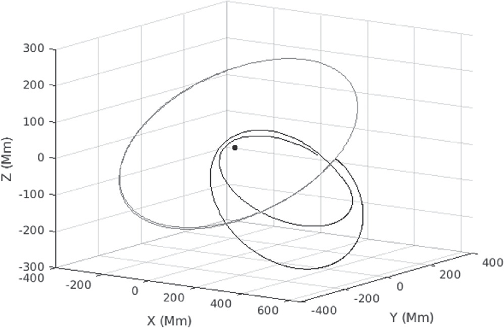
Figure 6. Example of the Chang'e 5-T1 R/B orbit (black curve) showing close approaches to the Earth between 2022 January until 2022 March, when it collided with the Moon, shown in the geocentric MEME J2000 equatorial reference frame. The Moon's orbit (gray curve) and Earth's location (black dot) are included for reference.
Download figure:
Standard image High-resolution imageUsing a sixth-degree zonal gravity model (Equation (4)), the trajectory of the Chang'e 5-T1 R/B can be precomputed before the actual Bayesian inversion process to reduce computation time. The requisite solar and observer positions at the appropriate observation epochs can also be precomputed to further improve efficiency. The short time window of observations and relatively large distance to the Chang'e 5-T1 R/B mean that higher-order perturbations (such as tesseral or sectoral harmonics) can be safely ignored during the trajectory integration. Since this Bayesian inversion model is very sensitive to attitude and reflective properties, any accuracy benefits from higher-order perturbations (including SRP) would be lost to the relative uncertainty of the inversion:

In Equation (4), U(r, θ, φ) is the generalized zonal gravitational potential of the Earth in spherical coordinates. When considering only zonal effects, the φ dependence reduces to the degree-dependent constants Al
and the θ dependence reduces to the generalized (associated) Legendre polynomials represented by  .
.
6.1.3. Reflective Dynamics
The simulated data used in the estimation process are a function of the location, shape, attitude, and reflective properties of the target body (Chang'e 5-T1 R/B), as well as the relative location of the Sun and observer (Linares et al. 2013). The simulated flux of the target at any instant in time may be calculated by:

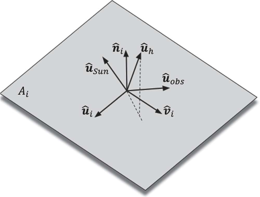
The total flux received by a sensor from the target, Ftgt, may be calculated as the sum of the flux from all facets of the target body. In this case, the target body is represented as a digital shape model described by many small triangular plates. A diagram of the layout of an individual body facet is given in Figure 7.

Figure 7. Illustration of the reference basis and relevant observation vectors on a shape model body facet.
Download figure:
Standard image High-resolution imageThe BRDF contribution, ρi
, from each facet is multiplied by the area of each facet, Ai
, projected in both the incident and reflecting directions (given by the dot products of the unit vectors in the Sun and observer directions with the surface normal). The flux density decreases with  , where d is the observer–target distance (Hinks et al. 2013). According to the modified Phong BRDF of Ashikmin & Shirley (2000), the total reflectance for each facet is the sum of the specular, ρs,i
, and diffuse, ρd,i
, components of the BRDF.
, where d is the observer–target distance (Hinks et al. 2013). According to the modified Phong BRDF of Ashikmin & Shirley (2000), the total reflectance for each facet is the sum of the specular, ρs,i
, and diffuse, ρd,i
, components of the BRDF.
Modeling anisotropy in the desired material can be controlled by the constants nu and nv , which influence the specularity in each facet direction (see Figure 7 for the facet basis definition and Campbell et al. 2022 for the specific form of the BRDF used):

The total flux calculated may then be used as in Equation (6) to calculate an estimated magnitude for the target object. The constant K is any calibration that needs to be applied. This calibration includes the zero-point offset for whichever spectral band or filter you are working with, as well as any noise, airmass extinction, or other effects being modeled that are not included in Ftgt. In this paper, K needs only to be set to the apparent solar magnitude in the appropriate filter for the observations being processed. See Section 2 for details on the filters used to collect observations.
6.2. Bayesian Estimation
In Bayesian statistics, the estimated posterior likelihood of an event is determined by any observational data available and any a priori assumptions about the system. Bayes' rule allows the estimation of the posterior conditional probability distributions  with the aid of a probabilistic model that associates all chosen parameters
θ
to observations
with the aid of a probabilistic model that associates all chosen parameters
θ
to observations  via a likelihood function (Aster et al. 2018):

The integral in the denominator of Equation (7) is just  and serves to normalize
  so that it may be considered a proper probability density function. Since direct computation of the posterior distributions for an arbitrary choice of parameters is challenging in a low-dimensional well-posed problem and impossible in an ill-posed problem, we employ a method known as MCMC sampling. This allows for the generation of values from an estimated posterior distribution that fits the observational data that you have and any a priori assumptions. The Metropolis–Hastings (MH) sampling method for MCMC simulations (Figure 8) is formulated so that the integral constant in the denominator of Equation (7) cancels out during the computation, allowing for the posterior distributions to be accurately estimated.

Figure 8. Brief overview of the MH algorithm for MCMC sampling.
Download figure:
Standard image High-resolution imageThis Markov chain method tests candidate samples with the acceptance probability α to ensure that the Markov chain tends toward areas of the parameter phase space with a higher posterior estimate. This means that we may use a computational model as described in Sections 6.1.1–6.1.3 together with an evaluation of the goodness of fit to the observed data (sum of square residuals) to evaluate the likelihood of each MH-generated sample from the parameter phase space,  . We may also supply an a priori estimate of the distributions to which our parameters belong (p(
θ
)), which can be uninformative (uniform distribution) if we have no strong a priori information.
. We may also supply an a priori estimate of the distributions to which our parameters belong (p(
θ
)), which can be uninformative (uniform distribution) if we have no strong a priori information.
While this method does produce a valid Markov chain, the Markov property is not what allows successful estimation of the posteriors. It is instead the fact that the estimated distributions are improved with each sampling, thus converging to the true distributions in the limit. Through continued generation of this Markov chain, we may accurately estimate the posterior distributions and only need to check the Markov chain for convergence to ensure a valid estimate of the posteriors.
7. Bayesian Analysis and Results
We ran a total of 100,000 iterations of our MCMC inversion on the data collected with the Leo-20 telescope on 2022 January 20 (see Table 2). Our prior distributions for each estimated parameter are partially uninformative, in that they are not true (infinite) uniform distributions, but rather finite distributions constrained by what is reasonable for both the model and the physics of the problem. A summary of the prior distributions for each parameter is given in Table 3. The parameters α and β describe the primary body axis orientation at the start of the observation epoch, w1−3 make the angular velocity vector, and ρ and F0 control the relative diffusivity and specularity of the body, respectively. Last, nu and nv control the amount of anisotropy in each of the body facet directions (see Figure 7).
Table 3. Partially Uninformative Prior Distribution for Each Parameter to Be Estimated by the Bayesian Inversion
| Variable | Initial Value | Min | Max | Distribution |
|---|---|---|---|---|
| α | 0.1 | 0 | 2π | U(0, 2π) |
| β | 0.1 | 0 | 2π | U(0, 2π) |
| w1 | 0.000 1 | −10 | 10 | U(− 10, 10) |
| w2 | 0.000 1 | −10 | 10 | U(− 10, 10) |
| w3 | 0.000 1 | −10 | 10 | U(− 10, 10) |
| ρ | 0.01 | 0 | 1 | U(0, 1) |
| F0 | 0.001 | 0 | 1 | U(0, 1) |
| nu | 10 | −1000 | 1000 | U(− 1000, 1000) |
| nv | 10 | −1000 | 1000 | U(− 1000, 1000) |
Download table as: ASCIITypeset image
As is the case for the majority of inverse problems of even moderate complexity, this estimation problem is ill-posed, so the results presented here represent a "best estimate." That is, due to the difficulty of sampling the complete surface of the Chang'e 5-T1 R/B and the large amount of symmetry on the rocket body, recovering the true states from this analysis is unlikely. However, there exist metrics that can be used to gauge the quality of the resulting estimates to provide confidence in the results.
By design, the MCMC estimation process is prone to getting "stuck" near the initial state estimation for some time. In order to ensure that the parameter space is diversely sampled and that we are not just sampling near our initial guess, we can look at the chain of all parameters chosen during the inversion process. This inertia-like property of MCMC algorithms is known as "burn-in" and is important to be aware of when using uninformative prior distributions. Looking at Figure 9, we see that the sampling chain, after the initial burn-in is removed, is highly varied and thus samples the parameter space sufficiently well.

Figure 9. Time history of parameter sampling from the Bayesian inversion where the first 55,000 samples have been removed to avoid burn-in.
Download figure:
Standard image High-resolution imageA quick quantitative way to evaluate the performance of the MCMC sampling is by checking the acceptance rate. Samples are only added to the posterior distribution estimate if they pass a strict sampling gate test. Ideally, the acceptance rate should be between 20% and 50% (Aster et al. 2018), and for our test we had an acceptance rate of 38.18%. If the acceptance rate is too low, then the estimation did not sufficiently sample the span of the parameter space and will not accurately portray the regions of highest posterior density (HPD). Conversely, if the acceptance rate is too high, then it is likely that the algorithm was stuck in a local extremum, and again we cannot be confident that it sufficiently sampled the span of the parameter space for globally valid results.
Figure 10 shows diagrams of the posterior distribution estimates for each parameter, and Table 4 summarizes the relevant parameters associated with the distributions for each parameter.

Figure 10. Final estimates of the posterior distributions of each parameter.
Download figure:
Standard image High-resolution imageTable 4. Bayesian and Frequentist Statistics for the Estimated Posterior Distributions of Each Parameter
| Variable | MAP | 95% HPD | Mean | STD |
|---|---|---|---|---|
| α | 0.002 | [0.0000, 0.0204] | 0.008 | 0.008 |
| β | 0.287 | [0.2473, 0.3008] | 0.282 | 0.013 |
| w1 | 0.000 | [–0.0001, 0.0001] | 0.000 | 0.000 |
| w2 | 0.000 | [–0.0001, 0.0001] | 0.000 | 0.000 |
| w3 | 0.017 | [0.0174, 0.0176] | 0.017 | 0.000 |
| ρ | 0.004 | [0.0025 0.0054] | 0.004 | 0.001 |
| F0 | 0.037 | [0.0276, 0.0500] | 0.037 | 0.006 |
| nu | 30.203 | [30.1695, 30.2221] | 30.197 | 0.013 |
| nv | 0.497 | [0.3995, 0.4999] | 0.465 | 0.030 |
Download table as: ASCIITypeset image
An important distinction for the values provided in Table 4 is the subtle difference between frequentist and Bayesian statistics as they are given here. The frequentist statistics (mean and standard deviation) are indicative of how often an event occurs, while the Bayesian statistics (maximum a posteriori, or MAP, and HPD) provide how likely it is that an event occurs, given the data you have and your understanding of the system. Looking at Figure 10 and comparing the values in Table 4, we see that in this case, the estimated distributions for our parameters can be well approximated by Gaussian distributions. This is typically not the case in general, as the estimated distributions from this process can be highly non-Gaussian.
Estimating the complete distribution of each parameter not only gives us insight into the global set of possible results, but also allows sampling from each distribution to evaluate behavior. In Figure 11, we took 1500 random samples from each distribution and fed them back into our forward model. Plotting the results and overlaying the raw Chang'e 5-T1 light curve, we can see that the estimated parameters and forward model fit the data very well. Note that the diagonal portion of the plot between 17 and 21 minutes post-epoch is when there were no data. Since it is possible for the "best estimate" to converge on an incorrect or poorly fitted solution, evaluating the results in this way offers a self-consistency check and confidence that the estimated parameters well describe the data.

Figure 11. The 97.5% HPD region (light gray) in light curve phase space as estimated by 1500 random samples from the posterior estimates generated with data taken from the Leo-20 telescope on 2022 January 20. The observed light curve of the Chang'e 5-T1 R/B has been overlaid in black. The diagonal portion of the light curve from approximately 17–21 minutes post-epoch is a period with no data.
Download figure:
Standard image High-resolution imageBased on the values in Table 4, it would appear that the Chang'e 5-T1 R/B is very anisotropic (ratio of nu
to nv
). As a reminder, these two parameters control the surface roughness and the degree of anisotropic reflection in either the  or
or  directions for each body facet (see Figure 7). In Table 4, we see that the estimated reflection is approximately 60 times greater in the
  direction than the
  direction. While it is quite likely that the Chang'e 5-T1 R/B exhibits some anisotropy, this level is unexpected. This result is likely due to the fact that the observations used for this estimation spanned a short time window, and so geometrically speaking, reflection in the orthogonal axis may not have been as visible. This is further supported by the rotation of the body being that of a very stable spin, implying that body surfaces are observed from the same geometry over short timescales as the body rotates. This is opposed to a complex tumbling body, where the observer–target body surface geometry may not be as periodic during rotation.
The strong periodic fits seen in Figures 5(a) and (b) imply that the Chang'e 5-T1 R/B was in a very uniform spin during the observations. This is reflected in our results by the estimated angular velocity (Table 4). Note that it is almost identically equal to a uniform spin about a single (the principal) body axis. This is somewhat unexpected for a typical rocket body, especially one that has been on-orbit for almost a decade and has had multiple close encounters with the Earth and Moon. In a typical (empty) rocket upper stage, the majority of its mass is concentrated toward the engines, giving an appreciable center-of-mass–center-of-figure (COM–COF) offset. This COM–COF offset can cause perturbations such as SRP or gravity gradient torque to have a larger destabilizing effect, giving rise to more complicated motion than just simple spin (i.e., precession, nutation, complex tumble, etc.; Takahashi et al. 2013), which is one possible explanation of the results seen in Campbell et al. (2022). However, we see no such evidence for perturbations in the spin of the Chang'e 5-T1 R/B, implying that the COM–COF offset may be smaller than expected. This would be the case if there was additional mass at the front of the rocket body, opposite the engines. This additional mass at the front of the body would bring the COM forward, closer to the COF, and thus reduce the effect of these destabilizing perturbations.
The Chang'e 5-T1 R/B hosted a secondary payload (in addition to the Chang'e 5-T1 spacecraft) that was comprised of two instruments and dubbed the Manfred Memorial Moon Mission by LuxSpace (Siddiqi 2018). This payload has a published mass of 10–14 kg and was permanently affixed to the front of the Chang'e 5-T1 R/B (Clark 2014; Moser et al. 2015; Siddiqi 2018). It is unclear if, or how, the upper stage was modified to accommodate this payload vis-à-vis structural support or additional equipment that might affect the final mass distribution, but the published mass of these instruments is only up to 14 kg, which is not enough to appreciably move the COM forward from the large mass of the dual-mounted YF-75 engines on its own (Cen et al. 2011).
One way to verify the hypothesis that there was additional mass in the front of the rocket body is to look for the crater that would result from the Chang'e 5-T1 R/B impact with the lunar surface. Craters have been found previously on the lunar surface following the impacts of rocket bodies from the Apollo missions. However, searching for a small impact crater among the plethora of craters on the Moon is challenging at best. Hence, predicting the precise location of the impact is critical for any hope of verifying this hypothesis.
8. Lunar Impact Location Prediction
The ephemeris of the Chang'e 5-T1 R/B was estimated by fitting orbits to right ascension and declination measurements reported by ground-based optical telescopes. A total of 508 observations were reported by 26 different stations from 2021 July 8 to 2022 February 10.
It was evident early on as observations accumulated that nongravitational accelerations had a significant effect on the trajectory. We used a typical radiation-based nongravitational perturbation model, where the accelerations radial, transverse, and normal to the heliocentric orbit are given in Equation (8) (Marsden et al. 1973):

A1, A2, and A3 are estimable parameters during the orbit fitting process. This model substantially improved fits over a purely ballistic trajectory, though it was nevertheless an imperfect match to the observations. This may have been due to outgassing from the rocket body or caused by a complex shape or rotation state. To limit the prediction errors stemming from the nongravitational perturbation model, we substantially shortened the fitted data arc, eventually settling on two orbit solution cases: one long and one short arc. After outlier rejection, the long arc included 162 observations spanning 57 days from 2021 December 15 to 2022 February 10. The short arc was of approximately half the duration, with 154 observations covering 28 days from 2022 January 13 to 2022 February 10. We also tested a simplified nongravitational acceleration model that included only the A1 term (representing SRP).
Figure 12 shows the predictions for these four test solutions, along with their associated 3σ uncertainty ellipses. The limited overlap among these solutions emphasizes the difficulty in nongravitational perturbation modeling. As a result, we elected to use the three-parameter nongravitational perturbation model in light of the optimistic uncertainties demonstrated by the one-parameter model. Thus, solution S23 was the final prediction, for which we document the orbital parameters in Table 5. The estimated radial term of the nongravitational acceleration model (A1) corresponds to an area-to-mass ratio of approximately 0.01 m2 kg−1. Based on the scatter among the predictions seen in Figure 12, we increased the impact location prediction uncertainties to ±4 km in longitude and +1/−3 km in latitude. Figure 12 also depicts the reported impact location from the Lunar Reconnaissance Orbiter (LRO), which indicates that the prediction was in error by 7.0 km in longitude and 2.7 km in latitude.

Figure 12. Impact prediction for several trajectory solutions as described in the text. The final delivered prediction was for solution "S23."
Download figure:
Standard image High-resolution imageTable 5. Estimated Nongravitational and Osculating Orbital Parameters for Solution S23 Giving the Predicted Lunar Impact Location
| Parameter | Value | 1σ Uncertainty |
|---|---|---|
| Epoch (TDB) | 2022 Feb 05 00:00:00 | N/A |
| a (km) | 321774.936 | 0.317 |
| e | 0.912983869 | 2.96E-7 |
| i (deg) | 31.4782088 | 4.52E-5 |
| ω (deg) | 151.4305753 | 8.02E-5 |
| Ω (deg) | 14.3057527 | 5.80E-5 |
| ν (deg) | 196.0218047 | 2.69E-5 |
| A1 (km s−2) | 42.597E-12 | 1.505E-12 |
| A2 (km s−2) | –1.808E-12 | 0.936E-12 |
| A3 (km s−2) | 2.079E-12 | 0.523E-12 |
Note. Osculating elements are given in the Earth-centered MEME J2000 equatorial reference frame.
Download table as: ASCIITypeset image
9. Impact Crater Morphology
Given the relatively high degree of certainty of the impact location of the Chang'e 5-T1 R/B on the lunar surface, there was a decent chance that it could be found. Fortunately, based on our predicted impact location, the LRO was able to find and image the impact site using the LRO narrow-angle camera (Robinson et al. 2010). Comparing LRO images of the impact site both pre- and post-impact gave rise to new questions. Instead of one round, or elongated, crater, such as what was seen when the Apollo Saturn IV-B rockets were sent into the Moon, there are two distinct craters side by side that were made by the Chang'e 5-T1 R/B. Figures 13(a) and (b) show the relevant section of lunar terrain both pre- and post-impact.

Figure 13. These are approximately 500 m sections of the lunar terrain captured by LRO showing the Chang'e 5-T1 R/B impact site and double crater that was formed. Before is from LRO image M1400727806L and after is from M1407760984R (NASA/GSFC/Arizona State University). Other visual differences in the terrain are caused primarily by the difference in the angle of solar incidence, which was approximately 28° during the before image and 59° in the after image. This section of terrain is near the Hertzsprung crater on the lunar far side.
Download figure:
Standard image High-resolution imageThe double crater (pictured in Figure 14) formed by the Chang'e 5-T1 R/B impact with the Moon was unexpected when considering what has been seen from other rocket body impacts with the Moon (Figure 15). Four Apollo Saturn IV-B rocket bodies were crashed into the Moon and created somewhat elongated craters, though they had shallow impact angles. The Chang'e 5-T1 R/B impact with the surface came from roughly 15° off vertical (75° impact angle), so that is not the case here. Moreover, the appearance of the craters is not of one elongated shape made from a single impact, but rather two distinct craters of similar size formed from separate impacts of similar energy. This supports our hypothesis that there was additional mass on the front end of the Chang'e 5-T1 R/B, creating the second crater during impact.
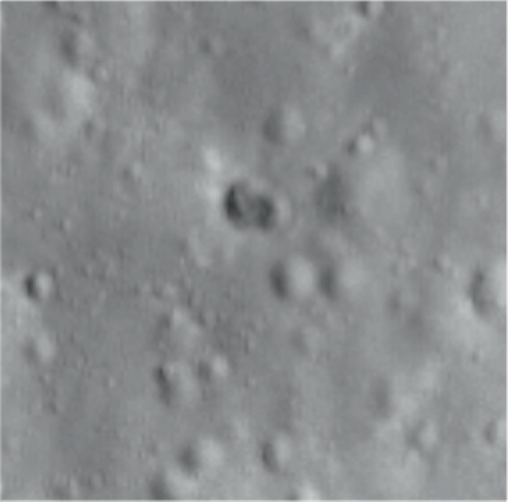
Figure 14. Zoomed-in view of the double crater formed by the Chang'e 5-T1 R/B impact with the Moon. Context images in Figures 13(a) and (b). Data from LRO image M1407760984R (NASA/GSFC/Arizona State University).
Download figure:
Standard image High-resolution image
Figure 15. Images of craters formed by the intentional impacts of the Apollo Saturn IV stages with the lunar surface. Note the round or elongated shapes, but all being explicitly one crater. (NASA/GSFC/Arizona State University).
Download figure:
Standard image High-resolution image
As noted earlier, there were additional instruments affixed to the front of the Chang'e 5-T1 R/B that were to stay attached to the rocket body post spacecraft detachment. The published mass of these instruments is only up to 14 kg (Clark 2014; Moser et al. 2015; Siddiqi 2018), which is not enough alone to account for the double crater seen post-impact.
10. Conclusions
In late 2021, it was discovered that an object (WE0913A) would impact the Moon in 2022 March after several close flybys of the Earth and the Moon over the coming months. The true identity of this object was up for debate, with two possibilities: (1) the Falcon 9 R/B from the DSCOVR mission; and (2) the Long March 3C R/B from the Chang'e 5-T1 mission. Our trajectory and spectroscopic analyses using ground-based telescope observations show conclusively that WE0913A is in fact the Chang'e 5-T1 R/B. Analysis of photometric light curves gave a spin period of 185.221 ± 6.540 s at a 1σ confidence level in the light curve of the Chang'e 5-T1 R/B just before the first close Earth flyby and a period of 177.754 ± 0.779 s at a 1σ confidence level just before the second close Earth flyby. Using MCMC sampling and a predictive light curve simulation based on an anisotropic Phong reflection model, we estimate both physical and dynamical properties of the Chang'e 5-T1 R/B at the start of an observation epoch. The Bayesian analysis implies that there was an additional mass at the front of the R/B that stabilizes the spin characteristics. We used the observations acquired to pinpoint the location of the impact on the lunar surface, which enabled the LRO to find and photograph the crater site. Our predicted location is within 7 km in longitude and 2.7 km in latitude from where the crater was eventually found by LRO. Comparing the pre- and post-impact images of the location shows two distinct craters side by side that were made by the Chang'e 5-T1 R/B. The double crater supports the hypothesis that there was additional mass at the front end of the rocket body, opposite the engines, in excess of the published mass of the secondary permanently affixed payload.
Acknowledgments
This work is supported in part by the state of Arizona Technology Research Initiative Fund (TRIF) grant (PI: Prof. Vishnu Reddy). A portion of this work was conducted at the Jet Propulsion Laboratory, California Institute of Technology, under a contract with the National Aeronautics and Space Administration.