


Abstract
Black hole (BH) environments often host plasmas that are fully collisionless or contain intrinsically collisionless regions, including relativistic jets and coronae, where particle energization is ubiquitous. Capturing the physics of these systems requires numerical methods capable of modeling relativistic, magnetized, collisionless plasmas in strong gravitational fields. In this work, we introduce the general relativistic module for Entity—the first open-source, coordinate-agnostic, performance-portable, particle-in-cell code. The code enables fast axisymmetric simulations of collisionless plasmas around BHs on any modern high-performance computing architecture (both GPUs and CPUs).

Original content from this work may be used under the terms of the Creative Commons Attribution 4.0 licence. Any further distribution of this work must maintain attribution to the author(s) and the title of the work, journal citation and DOI.
1. Introduction
Black holes (BHs) are fundamental astrophysical objects whose influence extends across a vast range of scales—from stellar environments to the intergalactic medium—where they play a central role in regulating the formation and evolution of cosmic structures. Because BHs cannot be observed directly, our understanding of them relies on interpreting their influence on the surrounding plasma, which typically consists of electrons, protons, heavier nuclei, and possibly positrons.
Significant progress in modeling such systems has been made through magnetohydrodynamic (MHD) simulations, which assume that the plasma is in local thermodynamic equilibrium. General relativistic MHD (GRMHD) further incorporates the effects of strong gravity, essential for accurately describing physics in curved spacetime (O. Porth et al. 2019). This framework has already yielded numerous insights into the global behavior of plasmas around BHs.
However, many phenomena associated with BHs remain poorly understood due to the numerical challenges involved in modeling the relevant plasma regimes. A prime example is the class of low-luminosity galactic nuclei, including M87* and Sgr A*, which have been imaged in unprecedented detail by the Event Horizon Telescope. These systems exhibit hot accretion flows (F. Yuan & R. Narayan 2014), where the plasma is essentially collisionless: the mean free path for Coulomb collisions exceeds the BH event horizon radius by about 6 orders of magnitude. Under such conditions, the plasma cannot easily thermalize, rendering the assumptions underlying MHD formally invalid. Nevertheless, MHD remains a valuable tool for capturing the large-scale dynamics governed by global conservation laws. Furthermore, additional justification for the fluid approximation can arise from effective “fluidization”—that is, effective collisionality induced by small-scale plasma instabilities.
In addition to their quiescent emission, many such systems display episodic flaring activity characterized by nonthermal spectra. For instance, Sgr A* produces bright, multiwavelength flares in the near-infrared, mid-infrared, and X-ray bands (K. Dodds-Eden et al. 2009; F. Yusef-Zadeh et al. 2009; GRAVITY Collaboration et al. 2018; S. D. von Fellenberg et al. 2025). Understanding these flares requires a detailed investigation of the dynamics during such episodes, the mechanisms responsible for the generation of nonthermal particles, and their resulting radiation.
Other regions of interest that are fundamentally collisionless exist in both stellar mass and supermassive BH systems. A notable example is relativistic jets, which, especially in the supermassive BH case, affect environments ranging from the immediate vicinity of the BH to the intracluster medium. Jet formation is widely attributed to the Blandford–Znajek (BZ) mechanism (R. D. Blandford & R. L. Znajek 1977), but interpreting their morphology and emission requires modeling pair loading, particle acceleration, and radiation mechanisms—processes beyond the scope of standard GRMHD.
Another example is the X-ray-emitting corona of efficiently accreting plasma flows, believed to be composed of a hot, magnetized, collisionless plasma located in the inner vicinity of the BH (A. A. Galeev et al. 1979; A. M. Beloborodov 2017; C. J. Bambic et al. 2024). The corona likely dissipates magnetic energy through a combination of magnetic reconnection and turbulence.
These considerations motivate the need for a framework that treats the plasma as collisionless while still incorporating the effects of strong gravity. Such an approach is realized through the general relativistic particle-in-cell (GRPIC) method, first developed by K. Parfrey et al. (2019). More recently, several new GRPIC codes have been introduced (A. Y. Chen et al. 2025; C. Meringolo et al. 2025). In this work, we present the first architecture-agnostic GRPIC code, which is publicly available as part of the Entity framework.7
The paper is structured as follows. In Section 2, we introduce the general equations in the 3+1 formalism and define our notation. Section 3 describes the numerical algorithm implemented within the Entity framework. Finally, in Section 4, we present a suite of test cases that validate our GRPIC implementation.
2. Equations in Curvilinear Spacetime
Throughout this paper, we use the following conventions: c denotes the speed of light and is taken to be 1 throughout this paper, G the gravitational constant, and M the mass of the central BH. We additionally define the gravitational radius as rg = GM.
The evolution of electromagnetic fields and charged particles in curved spacetime is naturally described using the 3+1 formalism. This approach foliates a Lorentzian manifold into a family of spatial hypersurfaces indexed by a global time coordinate. Extensive treatments of the formalism can be found in S. S. Komissarov (2004a), K. S. Thorne & D. MacDonald (1982), I. Y. Dodin & N. J. Fisch (2010), and E. Gourgoulhon (2012).
2.1. Spacetime Metric
We adopt the 3+1 decomposition of spacetime, where the manifold is endowed with a symmetric, nondegenerate metric tensor gμν of signature (− + + +), and restrict our analysis to stationary spacetimes. Throughout this work, Greek indices (μ, ν, …) run from 0 to 3, while Latin indices (i, j, …) range from 1 to 3 and denote spatial components.
A key component of the 3+1 formalism is the introduction of a time-like unit normal vector to the spatial hypersurfaces, which we define as

where α is the lapse function, encoding the proper time separation between hypersurfaces. This vector represents the covariant four-velocity of a local fiducial observer (FIDO). The spatial metric on each hypersurface—also referred to as the projection tensor—is given by

and has a Euclidean signature ( + + + ). It defines distances and inner products on the three-dimensional spatial slices.
The contravariant form of the FIDO four-velocity is

where βi is the shift vector, which describes the relative motion of the spatial coordinates with respect to the FIDO frame. The shift vector captures the nonorthogonality between the time coordinate and the spatial hypersurfaces. A useful identity relates the determinants of the full spacetime and spatial metrics:

With these definitions, the spacetime interval in 3+1 formalism reads

where β2 = βiβi, t is the coordinate time, and xi denotes the spatial coordinates.
Up to this point, all expressions assumed a general foliation of a Lorentzian manifold. In the case of a rotating Kerr BH, various foliations (and thus coordinate systems) are possible; in this work, we adopt Kerr–Schild coordinates to describe rotating Kerr BHs. This coordinate system is widely used in numerical simulations of accretion flows due to its regularity at the event horizon (while other coordinates, such as the Boyer–Lindquist system, introduce coordinate singularities near the horizon). Details of the Kerr–Schild metric, including its components, derivatives, and coordinate transformations, are provided in the Appendix.
2.2. Electromagnetic Fields and Maxwell’s Equations
The covariant Maxwell tensor is defined as

where Aμ is the electromagnetic four-potential, where, for visual clarity, we employ ∂μ ≡ ∂/∂xμ. The dual Maxwell tensor, often referred to as the Faraday tensor, is given by

where  , and εαβμν is the totally antisymmetric Levi–Civita symbol in four dimensions. In three spatial dimensions, we also define
 , where εijk is the 3D Levi–Civita symbol. For covariant components, the following identities hold:

Maxwell’s equations in covariant form are

where Iα = (ρ, J)T is the four-current density, containing the charge density ρ and the spatial current density J. To obtain Maxwell’s equations in a more familiar form, we define the spatial components of the electromagnetic field as

which allows us to recover the familiar special relativistic (SR) forms of Faraday’s law and the absence of magnetic monopoles from ∇β *Fαβ = 0:


where bold symbols denote contravariant 3-vectors, e.g., B ≡ Bi. From these, we also find

To express the second set of Maxwell’s equations in the 3+1 form, we additionally define

These definitions yield Gauss’s and Ampère’s laws


from which charge conservation naturally follows.
By construction, the vectors Bμ and Dμ are spatial; they lie within each spatial hypersurface and are orthogonal to the normal vector nμ, satisfying

Thus, B and D are treated as the primary fields, while E and H are considered auxiliary fields. The relationships between them is given by the following equations:

where α is the lapse function and β is the shift vector in the 3+1 decomposition of spacetime. In what follows, we simplify all our expressions assuming  , which is appropriate for the Kerr–Schild coordinate system. These relations, along with the spatial metric hij, encapsulate all gravitational effects in the 3+1 formulation of Maxwell’s equations. In the SR limit where α = 1 and β = 0, these reduce to the familiar flat spacetime electromagnetic fields:

2.3. Particles
In Lagrangian formulation, the equation of motion for a particle of mass m and charge q, moving in a curved spacetime under the influence of an external electromagnetic field, is given by

where xμ is the coordinate of the particle, τ is the particle’s proper time, and  are the Christoffel symbols (S. Weinberg 1972). The left-hand side describes the geodesic motion of a free particle in curved spacetime, accounting for gravitational effects via the Christoffel symbols. The right-hand side represents the Lorentz force acting on the particle, generalized to curved spacetime using the covariant Maxwell tensor Fμν.
Using 3+1 decomposition of the Maxwell tensor and Hamiltonian formulation, these equations can be written in the following form:
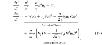
where t ≡ x0 is the coordinate time, (u0, ui) is the particle’s covariant four-velocity,8 and the FIDO-measured dimensionless energy, γ, can be found as

Additionally, in the Hamiltonian formulation, two useful conservation laws naturally arise. The conjugate four-momentum of a charged particle is defined as

where uμ is the four-velocity, Aμ is the electromagnetic four-potential, and pμ = muμ is the mechanical four-momentum. In spacetimes that admit time-translation and azimuthal symmetries, the corresponding conserved quantities are the total energy  and the angular momentum
 , given by


3. Particle-in-cell Algorithm in Curvilinear Space
Entity solves the Vlasov–Maxwell system of equations in flexible coordinates, by integrating the time-dependent Maxwell’s Equations (11) and (15) sourced by the currents imposed by macroparticles, which obey the equations of motion given by (19). Here, we describe the numerical algorithms and their implementation specific to the general relativistic (GR) module of the code. The current version supports 2.5D axisymmetric simulations in spherical coordinates, with a strong emphasis on simulations of BH magnetospheres and accretion. Full 3D simulations using the cubed-sphere grid will be presented in a future publication.
In what follows, we adopt code units, following the notation described in H. Hakobyan et al. (2026; hereafter Paper I). The physical coordinates are mapped onto code coordinates such that the grid is uniform in the code space. Consequently, the code coordinates span a range from zero to the total number of grid cells in each dimension, Nθ and Nr, for the radial and azimuthal axis, respectively. Any offset from the grid nodes is represented by the displacement from the corner of the cell, denoted as dx. The position of each particle is stored using two quantities: the index of the cell it occupies and the displacement within that cell (e.g., i1 and dx1); see Paper I for details of the coordinate implementation. The components of the spatial metric hij are expressed in normalized code units (see the Appendix). Unlike the SR module, the GR module assumes that the magnetic and electric field components supplied by the problem generator are already given in code units (the spatial staggering of each component is still done by the code automatically). This convention is convenient, as field quantities are often initialized using combinations of metric components.
We employ a finite-difference time-domain leapfrog scheme, discretizing both the electric Di and the magnetic Bi fields in both time and space. As in SR, electric field components and particle positions are defined at integer time steps, (n)t, while magnetic fields and particle four-velocities are staggered by half a time step back, (n–1/2)t. Typewriter font (e.g., i, n) denotes indices on the discretized numerical grid in both time and space. The time step is fixed, Δt ≡ (n)t − (n-1)t, such that (n)t ≡ nΔt.
Implementation in GR largely follows the SR structure. However, because D and B fields are coupled via the auxiliary fields E and H, the leapfrog algorithm requires modifications: copies of fields and electric current at two different times are stored (more details to follow in Section 3.4). Some field components must be interpolated to grid positions not defined on the Yee mesh (see Section 3.3.1), and the electric current deposition requires storing both the initial and the final particle positions (Section 3.2).
3.1. Particles
We solve the equations of motion for macroparticles given in (19). Particle coordinates and velocities are staggered in time using a second-order accurate leapfrog scheme. In this approach, the velocity is advanced first and then used to update the position. At time step n, the velocity is updated from (n–1/2)ui to (n+1/2)ui, after which the position is advanced from (n)xi to (n+1)xi

The velocity update is performed using symmetric second-order accurate Strang splitting (K. Parfrey et al. 2019)

where  and
 denote the pure geodesic and electromagnetic update operators, respectively. These correspond to the “curvature” and Lorentz force terms in (19).
The electromagnetic stage of the particle pusher implemented in the GRPIC module follows the standard Boris algorithm, as described in Paper I, which is widely employed in flat spacetime particle-in-cell codes for its numerical stability and excellent long-term behavior. The principal modification for the GR case is the inclusion of a tetrad transformation that maps the particle velocity and electromagnetic field components from the global coordinate basis to a locally flat orthonormal frame. This transformation is applied at the beginning of each velocity update half step in  , enabling the use of the SR Boris procedure in the local frame. After the push, the updated velocities are transformed back to the global coordinate basis using the inverse tetrads.
For the geodesic update, we employ an iterative midpoint integrator to advance both the velocity and the position of the particle. In this scheme, the new velocity (or position) is first predicted using an initial guess and then iteratively corrected based on the updated local metric quantities. For the geodesic velocity update, let (n–1/2)ui denote the components of the covariant four-velocity of the particle before the update. The initial guess (zeroth iteration) for the advanced velocity is taken as  , and the solution is iteratively refined according to

where the solution approaches the exact value,  , as the number of iterations, m, grows. In practice, convergence of the iterative scheme is typically achieved within ten iterations; the fixed number of iterations, niter, is a user-configurable parameter. The explicit form of the geodesic velocity update during each iteration is given with the following relation:
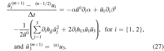
Here,  , and
 is the FIDO-measured energy associated with the four-velocity
 . The exact analytic expressions for the derivatives of the metric components are used in the integration and are provided in the Appendix. Since the GR push is performed after the half of the electromagnetic push (which is described in detail below), for the massive charged particles, this initial velocity guess in the former corresponds to that obtained after the first electromagnetic half push,
 , while for the chargeless particles, the EM push is skipped altogether. The velocity update involves coordinate-dependent metric coefficients computed at the position of the particle. Because our algorithm implements a leapfrog scheme, we use the position from the previous time step, (n)xi, for the metric coefficients in (27).
The newly obtained velocity may then be used to update the particle’s position, which we also perform iteratively. Given the previous time-step position, we take the initial guess as  , and iterate according to

The full expression according to Equation (19) takes the following explicit form

In Equation (29), all the metric coefficients, as well as the α and βi are computed at an intermediate position,  .
Although our algorithm does not strictly require it, we also record the out-of-plane angular coordinate, x3 ≡ ϕ, for each of the particles. This quantity is mainly used to test the particle pusher, as described in Section 4. After each push, the coordinate is updated based on the newly computed velocity according to

Below we describe the full numerical scheme for a single particle update at a time step n.
- 1.Save previous location:
 .
- 2.Interpolate field components to the particle’s initial location:, .
- 3.Transform the interpolated fields as well as the particle’s velocity to the tetrad basis:,
.
- 4.Perform the first EM push (in tetrad basis) for Δt/2:.
- 5.Transform the partially updated velocity back to the covariant basis at (n)xi:.
- 6.Perform the implicit geodesic velocity update at fixed (n)xi:.
- 7.Transform the updated velocity back to the tetrad basis at (n)xi:.
- 8.Perform the second EM push (in tetrad basis) for Δt/2:.
- 9.Transform the updated velocity to covariant basis at (n)xi; this completes the velocity half of the leapfrog update:.
- 10.Perform the implicit geodesic coordinate update (full Δt):.
- 11.Update the out-of-plane coordinate using (30):.



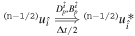
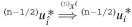
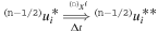

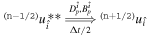

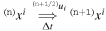
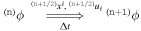
Steps 4–6 and 8–10 are part of the EMpush routine within the particle pusher kernel of the GR module. The geodesic velocity and coordinate updates are performed by the GeodesicMomentumPush and GeodesicCoordinatePush routines, respectively. For the massless particles, the EMpush routine is skipped.
3.2. Electric Currents
We derive the charge continuity equation by taking the divergence of the covariant Ampère’s law and using Poisson’s law:
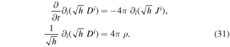
Here, ρ denotes the charge density. Therefore, the charge conservation takes the same form as in special relativity (see Paper I):

As discussed in Paper I, we employ a coordinate-conformal particle shape function  and deposit conformal currents
 on the grid. Here, xi denotes the grid coordinate, and
 is the position of each macroparticle. The total charge density contributed by all particles at a given location is

where ∑p runs over all particles of species s, and ∑s is the sum over all species. Then the time-discretized form of the current deposition is given by

Thus, the current deposition and filtering routines are identical to those used in the SR curvilinear module.
From Equation (34), it follows that only the initial and final particle positions,  and
 , are required for the current deposition. In explicit particle-in-cell (PIC) schemes, the final position is known, and the initial one can typically be inferred as

However, in Entity, this approach cannot be used, and the initial positions must instead be stored explicitly.
For the out-of-plane current density, on the other hand, we can compute its value directly, using the following formula:

which is identical to the SR expression, except for the inclusion of the lapse function α ≠ 1.
3.3. Field Solver
In 3+1 formulation, the electromagnetic field evolution is written in covariant form as
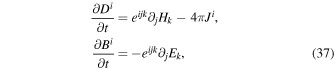
with the auxiliary fields determined as

where  and εijk is the Levi–Civita symbol.
Compared to SR PIC, GR evolution requires storing additional time-shifted field states for interpolation and time centering. In Entity, the arrays denoted as em0 (see Paper I for more details on how the fields are stored) correspond to (n-3/2)Bi and (n-1)Di, while the auxiliary arrays, aux, store (n-1/2)Hi and (n)Ei. Currents are defined at (n+1/2)Ji (computed from particle positions  and
 ) and we also retain the previous-step currents, cur0, (n-1/2)Ji. Because Hi and Ei depend both on Bi and Di, the magnetic and electric field updates are coupled and must be known simultaneously to calculate the auxiliary fields, complicating the canonical leapfrog update (K. Parfrey et al. 2019).
3.3.1. Spatial Discretization
The spatial discretization of Bi, Di, and Ji is done according to the Yee scheme (K. Yee 1966), with auxiliary fields Hi and Ei discretized in the same manner as the primary fields. In the Yee mesh, the electromagnetic fields Bi and Di are defined at different spatial locations, requiring interpolation to a common location for the computation of Hi and Ei, in addition to interpolation in time. An additional complication arises from the presence of a nondiagonal spatial metric, which requires interpolation of different components of the same field. The computational grid is uniform and equally spaced in the general code coordinates. The spacetime geometry is specified by the metric coefficients.
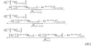
In this section, we present the discretized forms of Faraday and Ampère routines, given by Equation (37), along with the computation of the auxiliary fields in Equation (38); see the right panel of Figure 1. Each of the Faraday and Ampère substeps in the cycle described in Section 3.2 is carried out in the same manner. The discretized Faraday closely resembles the curvilinear SRPIC version described in Paper I, but here includes the additional contributions due to the nondiagonal metric.
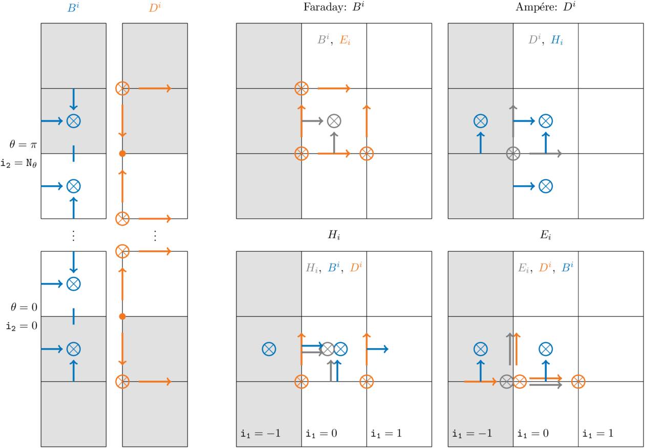
Figure 1. Left: locations of Bi and Di components for which boundary conditions on both of the axes are defined. The solid (no arrow) lines for  ,
 , as well as solid circles for
 , and
 indicate that these components are set to zero by symmetry. The other components are either reflected exactly (r-components) or reflected with the opposite sign (θ-components). Right: location of the components of electromagnetic fields used for each of the four main routines. The deduced components for the cell (i1 = 0, i2) are shown with gray. All the magnetic and electric field components used in the respective routines are shown in blue and orange, respectively.
Download figure:
Standard image High-resolution imageIn the equations below, we use the following conventions for brevity:
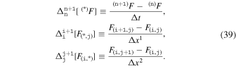
The following describes the main Faraday update (see step 6 in Section 3.4):
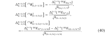
The update due to Ampère’s law (see step 7 in Section 3.4), where  is the deposited conformal currents, is
The spatial discretization of the auxiliary electric field Ei and magnetic field Hi is given by
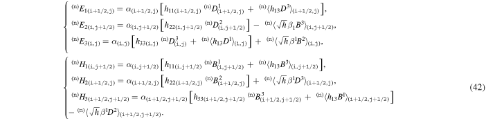
Here, the quantities enclosed in angular brackets 〈·〉 are not defined exactly at the locations where they are required and therefore must be interpolated. We perform this interpolation using a volume-weighted averaging scheme. For any quantity a, the value at a grid point (i, j) is computed as

Therefore, the value of a at a radial location i is obtained from its neighboring values at i-1 and i + 1, weighted by their corresponding cell volumes V(i±1,j). The volume of a computational cell is given by  , where dx1 = dx2 = 1 for our choice of a uniform grid spacing.
The explicit form for the interpolated quantities in (42) is then
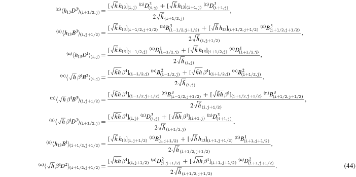
Here,  , which is used as an auxiliary to avoid finite-precision errors; notice that we are able to use this definition since both the numerator and the denominator in all the relations from (44) are defined at the same θ-position, i.e., the same index j, and the potentially problematic
 from the metric cancel out analytically.
3.3.2. Special Treatment of the Polar Axes
Spherical coordinates contain a coordinate singularity at the axes (θ = 0 and θ = π), where the metric determinant vanishes ( ). This raises an issue of how to evolve quantities defined exactly on the axes: in our discretization, these are the components D1, D3, and B2. First of all, the θ and ϕ components of the field must vanish by symmetry—these boundary conditions are described in detail in the next section. Consequently, we do not evolve D3 and B2 on the axes.
The component D1, however, remains nonvanishing and must therefore be explicitly accounted for in Ampére’s law. We impose zero-gradient boundary conditions on D1 at the axes.9
Accordingly, in a cell adjacent to the axis at θ = π (i2 = Nθ), we set  , while in a cell adjacent to the axis at θ = 0 (i2 = 0), we set
 .
Exactly on the axes, the metric component h33 becomes singular, which can lead to numerical issues in the geodesic pusher when particles approach the axis too closely (due to finite numerical precision). In practice, this situation occurs rarely—typically for only a few particles (out of billions) with nearly vanishing toroidal velocity. For such cases, at the beginning of each push, the particle's physical coordinate x2 is replaced with the value stored as SMALL_ANGLE_GR ≈ 10−5 (a compile-time definition) to avoid the singularity and ensure stable integration. The same regularization procedure is applied during the deposition of the out-of-plane current component,  , where the same coordinate replacement is used for evaluating the particle’s u3 velocity component.
3.3.3. Boundary Conditions
Boundary conditions are imposed on evolved electromagnetic field components, em, only. Under axisymmetry, fields in the ghost zones adjacent to the axis satisfy reflection symmetry (see the left panel of Figure 1). At the outer boundary, the fields are matched to their initial values using an absorbing layer (see MATCH boundaries described in Paper I). Both the axial and the outer boundary conditions are identical to those in SR and are handled by the same routines.
The treatment for the particles, however, is different, since in SR their positions are updated in the global Cartesian basis, where the axis is not present. In GR, particles are “reflected” from the axes once their inferred coordinate lies outside the block: if i2 < 0 or i2 ≥ Nθ (with i2 being the integer component of the particle position in code units). In that case, the cell index of the particle is reset to i2 = 0 or i2 = Nθ−1, while the subcell displacement is updated as dx2 → 1 − dx2, and the tangential velocity, u2, is inverted, u2 → −u2.
The computational domain extends inside the event horizon, where we impose constant boundary conditions for the electromagnetic fields. Specifically, all the field components in the layer of cells from i1 = −N_GHOSTS to i1 = nf are set equal to their corresponding values at i1 = nf + 1. Here, nf denotes the number of current filters applied. This treatment prevents filtered currents associated with particles removed within the horizon from coupling back into the physical domain. Consequently, the inner boundary of the computational domain must always be placed at least nf + 1 cells inside the event horizon. Particles are allowed to cross the horizon freely and are removed from the computational domain once they pass through the layer of cells where constant boundary conditions for the fields are applied and enter the ghost zone.
3.4. PIC Loop
Each time step proceeds according to the following scheme:
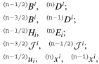
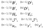
- 1.Start at (n)t with the following quantities stored:where xi and ui are the particle’s coordinates and velocities, respectively.
- 2.As in SR, we need to align Bi and Di in time for the subsequent particle push, as both fields are part of the Lorentz force. This is done via several steps:
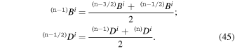
- a.Interpolate Bi and Di to an intermediate time:
- b.Compute the auxiliary field Ei at (n-1/2)t:
- c.Perform an auxiliary Faraday substep to update the interpolated magnetic field (n-1)Bi:
- 3.Using (n)Bi and (n)Di, we can now push the particles as outlined in Section 3.1:
- 4.Using the initial and final locations of particles, the conformal current deposition is performed:
- 5.We then compute the midpoint values for the electric currents:
- 6.Perform the full Faraday update for the Bi:
- a.Compute auxiliary fields at (n)t:
- b.Perform the main Faraday update:
- 7.Perform the update of the Di field via two Ampère substeps:
- a.Perform an auxiliary Ampère substep:
- b.Recover auxiliary field Hi at (n+1/2)t:
- c.Perform the final Ampère substep:
- 8.Finally at (n+1)t we have the following quantities:and the loop is repeated.










3.5. Comment on the Performance
Many of the GR routines are shared with the main SR module of the Entity described in detail in Paper I. For example, the current deposition routine for the conformal electric currents is identical. The field-evolution algorithm is also the same, except that in GR it is executed twice per time step and additionally includes the recovery step for the auxiliary fields. The principal differences from the performance standpoint thus lie in the particle pusher, and in the amount of data—for both the particles and fields—that must be communicated between the meshblocks in multi-GPU runs. In terms of the memory footprint, the GR module also stores 3 times as many electromagnetic field components (including the auxiliary fields, the additional fields at staggered time steps, as well as the electric currents at a previous time).
We benchmarked each major algorithmic component on a single NVIDIA A100 GPU using the monopole test (Section 4.5) performed with a 20482 mesh which is logarithmic in r and linear in θ hosting 90 particles per cell. With a well-balanced load, the particle pusher dominates the time step at about 6.2 ns per particle; the field solver requires 2–3 ns per cell each step (which is typically negligible with a high number of particles per cell). For reference, in the 2D SR tests of Paper I, the pusher and current deposition each cost ≈1–2 ns per particle, with the pusher again being the most expensive kernel. Communication costs on multi-GPU runs are dominated by particles and are thus identical to those reported in Paper I (since the particle arrays are identical). The current deposition cost is identical to that in SR.
4. Tests
In this section, we first describe the tests used to validate each routine of the scheme individually. We then present test simulations of the full PIC scheme, comparing our results with both previous studies in the literature and analytic solutions available in the force-free regime.
4.1. Pusher
To validate the particle pusher, we separately test its geodesic and electromagnetic components, and then test the full scheme by reproducing results reported in the literature. Table 1 summarizes the orbits considered in this subsection, specifying the magnetic field configuration, the BH spin, and the initial orbital parameters (including the energy  , the angular momentum
 , the coordinates r and θ, and the initial velocity components). All the orbits are shown in Figure 2 (top row) with their respective relative errors shown in the bottom row.
Table 1. Summary of the Test Particle Orbits Shown in Figure 2
| Name | Field | a |

| N | Δt/(rg) |

|

| r/rg | θ | u1 | u3 |
|---|---|---|---|---|---|---|---|---|---|---|---|
| GR | zero-field | 0.995 | 15 | 512 | 0.01 | 0.92025 | 2 | 10.6498 | π/2 | 0.18915 | 2.0 |
| SR-EM | Wald a = 0 | ⋯ | 20 | 1024 | 0.01 | 1.41421 | 10.0 | 10.0 | π/2 | 0 | 10.0 |
| GR-EM-2D | Wald a = 0 | 0.0 | 20 | 1024 | 0.01 | 0.873 | 4.5 | 4 | π/2 | 0.873 | 2.9 |
| GR-EM-3D | Wald | 0.9 | 8 | 1024 | 0.001 | 2.2226 | 18.10399 | 4 | π/2 − 0.2 | 0.5664 | 2.361 |
Note. The simulation setup is specified by the field configuration, black hole spin a, outer boundary position, and the number of grid cells (identical in the r and θ directions in all cases). The normalized components of the four-velocity are listed in Kerr–Schild coordinates, with u2 = 0 for all cases.
Download table as: ASCIITypeset image
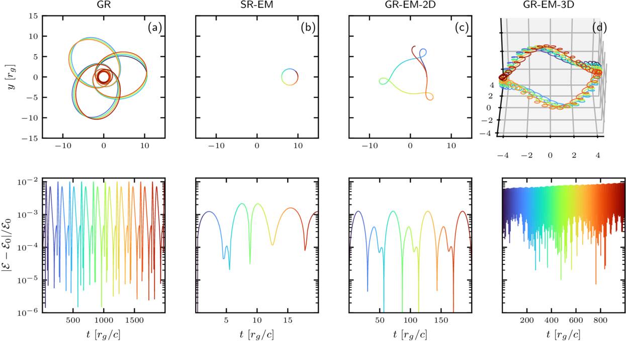
Figure 2. Test particles’ orbits (top row) and their corresponding relative energy errors (bottom).
Download figure:
Standard image High-resolution imageInitial conditions of all particles for the tests presented below are characterized by  , the condition that u1,BL = u2,BL = 0 (where the subscript “BL” means the velocities measured in Boyer–Lindquist coordinates, whereas “KS” will denote those in Kerr–Schild coordinates10
), and the θ coordinate. From these quantities, the values for u0,BL = u0,KS and
 can be deduced. For comparison with our Kerr–Schild framework, the corresponding covariant velocity components can be found using the following:
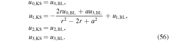
The coordinate positions themselves remain unchanged. Below, we ignore the “KS” subscript for brevity, implying that all the quantities are in Kerr–Schild coordinates.
The initial radial coordinate is determined from the energy  via the normalization of the four-momentum for massive particles

which yields a relation via quadratic equation between the particle’s coordinates, velocities, and its energy in KS coordinates:

where A ≡ g00, B ≡ −2g01u1, and  . Here the sign is chosen such that
 . To assess numerical accuracy over time, we monitor the relative error in energy,
 , where
 is the initial orbital energy. Small discrepancies with published test particle trajectories can arise even for apparently identical initial conditions because our integrator is time staggered: coordinates and velocities are offset by half a time step. For this reason, when evaluating
 we align variables by taking the position at the velocity time level, i.e., the midpoint (average) of the position at the adjacent time steps.
4.1.1. Geodesics Force
We first reproduce the three-leaf orbit described in J. Levin & G. Perez-Giz (2008) (see their Figure 15, also reproduced in M. Zou et al. 2025) as a demonstration of our geodesic pusher (Figure 2(a)). We use a time step of Δt = 0.01 rg and evolve the orbit up to 2000 rg. We successfully reproduce the orbit, which exhibits a small precession, and while the energy error grows as the particle approaches pericenter. The error remains stable and bounded over long timescales (Figure 2(a) bottom).
4.1.2. Lorentz Force
We now turn to orbits in the presence of a magnetic field. The Wald solution (R. M. Wald 1974) describes an electromagnetic four-potential corresponding to a magnetic field aligned with the BH spin axis that is uniform at spatial infinity. In Kerr–Schild coordinates, the vector potential Aμ defining the zero-charge solution is
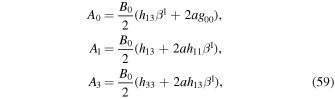
where B0 is the asymptotic magnetic field strength. To set this field in the code, we compute Bi according to Equation (12), and then compute gravitationally induced Di in KS coordinates.
To test the electromagnetic pusher in isolation, we consider the general relativistic metric with flat spacetime (no gravity, and a = 0), which is mathematically equivalent to a spherical grid modeled using the SR module (for convenience, we still measure temporal and spatial dimensions in rg which in this case bears no physical meaning, i.e., the metric does not depend on its value). In this case, the magnetic field reduces to a uniform vertical field (in the r–θ plane). This setup allows us to test simple particle gyration in a nontrivial coordinate system, requiring transformations between covariant components and the tetrad frame. The orbit, shown in the second column of Figure 2, is initialized in a vertical field with fiducial Larmor radius ρ0 = 2 rg (see Paper I for details on code units and magnetic field normalization), using a time step Δt = 0.01 rg.
This setup corresponds to a physical Larmor radius of the particle of  , as illustrated in Figure 2(b). The trajectory remains closed and the energy error stays bounded (Figure 2(b) bottom).
4.1.3. Full Pusher
We now test the full pusher scheme for an orbit in the r–ϕ plane for the nonspinning case (a = 0). The results of numerical integration are shown in Figure 2(c). We initialize the magnetic field according to the Wald’s solution, as given by Equation (59), which corresponds to a purely vertical uniform magnetic field in Boyer–Lindquist coordinates. However, in Kerr–Schild coordinates, a nonzero electric field arises from the coupling of the shift β1 with B2. As a benchmark, we reproduce one of the charged-particle orbits reported in M. Kološ et al. (2015). For a vertical field, the conjugate angular momentum includes the magnetic field contribution; hence, for a nonspinning BH, the toroidal velocity can be inferred from

We reproduce the orbit presented in Figure 6.2 of M. Kološ et al. (2015). To match the magnetic field normalization for  , we adopt the fiducial Larmor radius
 , corresponding to ρ0 = 5 rg for q/m = 1 and
 .
Following Z. Stuchlík & M. Kološ (2016), we validate fully three-dimensional test particle trajectories in the analytic vacuum Wald magnetic field (Equation (59)) for a Kerr BH with a dimensionless spin a = 0.9 (with the magnetic field aligned with the spin axis). Figure 2(d) reproduces Figure 11 (right column) from the same authors, showing a regular (nonchaotic) orbit. We adopt their normalization  , corresponding to a fiducial Larmor radius ρ0 = 0.5 rg. To initialize the orbit, we treat the particle as neutral on a Keplerian trajectory: we take ut and uϕ from Equations (63)–(64) of Z. Stuchlík & M. Kološ (2016) and obtain the corresponding Kerr–Schild radial component ur via Equation (56). Note that similar orbits were studied by F. Bacchini et al. (2019) and A. Y. Chen et al. (2025), albeit with different initial velocities. In contrast to the other orbits discussed above, we observe a slow, monotonic drift in the relative energy error. However, the error remains small and bounded. This secular trend is due to the interpolation of the spatially varying magnetic field (see also F. Bacchini et al. 2019).
4.2. Wald Solution in Vacuum
We now test the evolution of electromagnetic fields in vacuum, i.e., in the absence of plasma. The problem generator for this test is included in Entity, with two available initial field configurations defined in the input file via the init_field setting, which can be set to either wald or vertical. The former initializes the fields according to Equation (59), while the latter corresponds to a purely vertical magnetic field—the zero-spin limit of Equation (59).
Figure 3 shows the evolution of the Wald solution in vacuum for a spin parameter a = 0.95. Each of the six panels represents one component of the electromagnetic field: the magnetic field (Br, Bθ, Bϕ) in the top row and the electric field (Dr, Dθ, Dϕ) in the bottom row. In each panel, the left half (x < 0) displays the initial condition, while the right half (x > 0) shows the state at t = 500rg. In the first panel, thin black lines overlay Br to illustrate the magnetic field lines. The simulation was performed at a resolution of 5122 with a grid uniform in θ and logarithmic in r. In the absorbing layer, we smoothly match the field components with the analytic solution. The solution remains stable and well preserved after ∼105 time steps, matching exactly the analytic expression.
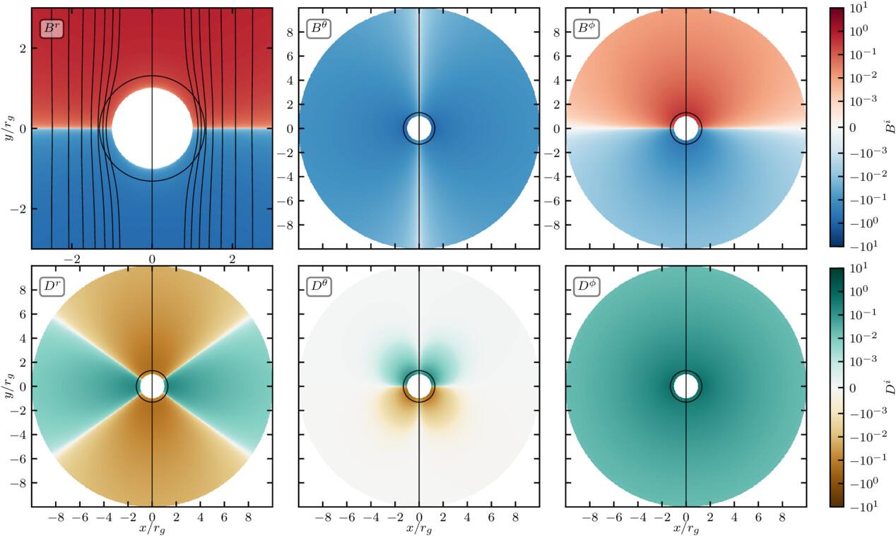
Figure 3. Conservation of Wald solution in vacuum, from the initial state (left side of each panel) to t = 250rg (right side of each panel). The top row shows the magnetic field components Bi, while the bottom row shows the electric field components Di. In the first panel, black contours trace the magnetic field lines and we show a zoom-in close to the BH. In all panels, the event horizon is indicated by a thin, round black outline.
Download figure:
Standard image High-resolution image4.3. Deposit
We next test the current deposition scheme in the presence of a rapidly spinning BH (a = 0.95). The system is initialized without any electromagnetic fields, and an electron–positron pair is placed at (r, θ) = (17 rg, π/2). The particles are given equal and opposite radial velocities, ur = +5 for the electron and ur = −5 for the positron. At the outer boundary, we impose reflection for the electron instead of absorption. As a result, both particles eventually fall into the BH, as illustrated in the snapshots of Figures 4(a)–(c), which show the particle trajectories superimposed on the evolving electric field distribution.
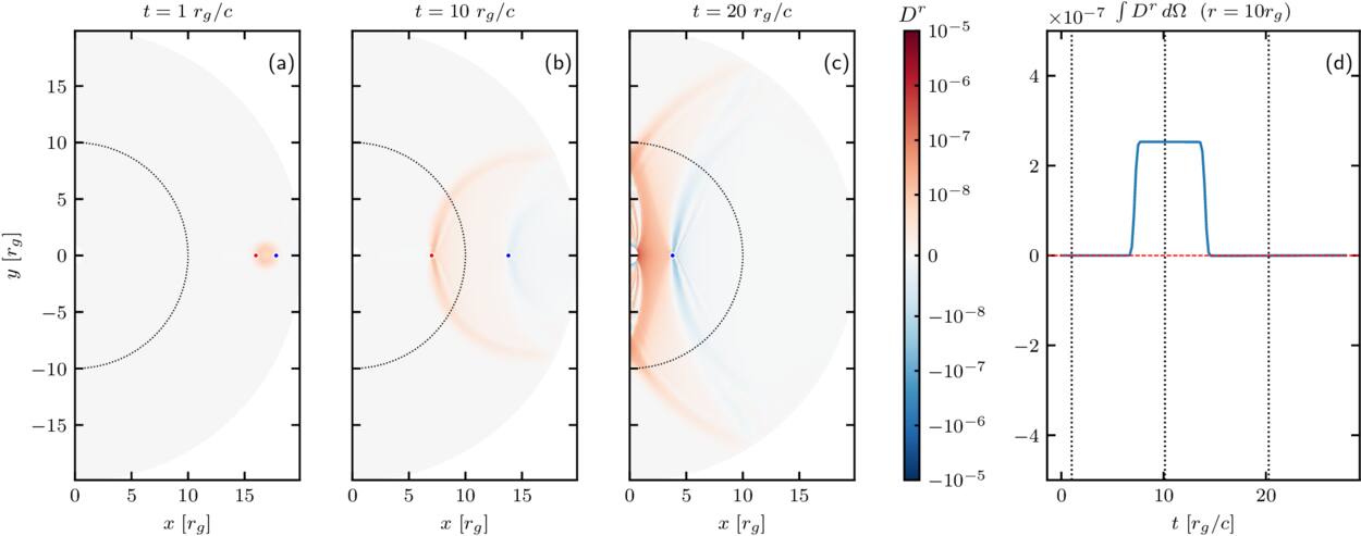
Figure 4. Panels (a)–(c): snapshots of the radial component of the electric field Dr (in color) at three different times (t = 1 rg, 10 rg, and 20 rg). The dotted semicircle indicates the reference radius r = 10 rg. The blue and red markers denote the two particles (electron and positron). Panel (d): time evolution of the angular integral ∫Dr dΩ at r = 10 rg, with vertical dashed lines marking the snapshot times.
Download figure:
Standard image High-resolution imagePanel (d) of Figure 4 shows the evolution of the flux of Dr, computed over a spherical surface at r = 10 rg. The integral initially increases as the particles move, but ultimately decays to zero, demonstrating perfect charge conservation.
4.4. Plasma-filled Magnetosphere
To validate the full PIC scheme, we reproduce the setup of K. Parfrey et al. (2019). Specifically, we initialize the Wald solution corresponding to a uniform vertical magnetic field around a rapidly spinning BH with spin parameter a = 0.95, and continuously inject plasma into the magnetosphere to replenish the lost plasma. Our computational domain extends to 6rg, with an absorbing layer beginning at 5rg. We use a grid of 20482 cells with logarithmic spacing in r. As plasma accretes, both the density and magnetic field strength increase, and the steady-state skin depth near the BH is established at ≈0.005 rg (the fiducial skin depth for n = n0 is taken to be d0 = 0.05 rg, while the fiducial Larmor radius ρ0 = 0.025 rg). The nominal number of particles per cell is nppc = 2, but the effective value is substantially higher owing to continuous plasma injection. Electron–positron pairs are injected with a temperature T± = 0.5m± whenever local magnetization exceeds σ ≡ BiBi/(4πn±m±) ≥ 1000. This setup corresponds to the standard accretion problem generator provided with Entity.
As the simulation proceeds, the magnetosphere rapidly becomes plasma-loaded. Figure 5 shows the state at t = 90 rg. With increasing plasma supply, the field lines deviate from the vacuum solution and bend toward the BH near and within the ergosphere. After roughly 10 rg, the system settles into a quasi–steady state characterized by an approximately monopolar poloidal field inside the ergosphere, and a persistent Y-point and current sheet. In this regime, the current sheet reconnects continuously and is susceptible to a drift-kink instability. The resulting plasma distribution exhibits the expected high-supply structure, consistent with K. Parfrey et al. (2019).
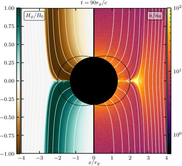
Figure 5. Snapshot of the plasma-filled magnetosphere around a rapidly rotating black hole (a = 0.95) at t = 90 rg. The color scales show Hϕ normalized to the fiducial B0 (left) and the plasma number density normalized to the fiducial density n0 (right). White curves indicate magnetic field lines. The black circle marks the event horizon, and the vertical solid line denotes the rotation axis. Continuous pair injection maintains densities at or above the Goldreich–Julian level, resulting in a filled magnetosphere consistent with the high-supply regime of K. Parfrey et al. (2019).
Download figure:
Standard image High-resolution image4.5. BZ Monopole
In this test we initialize a zero-spin magnetic monopole solution centered on the BH, reproducing the classic BZ solution (R. D. Blandford & R. L. Znajek 1977; see also S. S. Komissarov 2001, 2004b for force-free and GRMHD extensions)

which yields  , with all other field components set to zero. The computational domain extends to
 , with an absorbing layer of 1 rg thick near the outer boundary. The resolution is 10242, and the BH spin is set to a = 0.2 (though we have also tested higher spins). The inner boundary lies at
 .
We adopt fiducial skin depths d0 = 2.5 × 10⁻³rg and ρ0 = 5 × 10⁻⁵rg, resulting in the value for the fiducial plasma magnetization of σ0 = 2500. Maxwellian plasma with T± = 0.5m± is injected wherever the local magnetization exceeds σth = 2000. The density profile follows n ∝ r−2 scaling. The choice of σth yields densities significantly above the Goldreich–Julian value, leading to high plasma multiplicity. The resulting Hϕ at 200rg is shown in Figure 6(a).
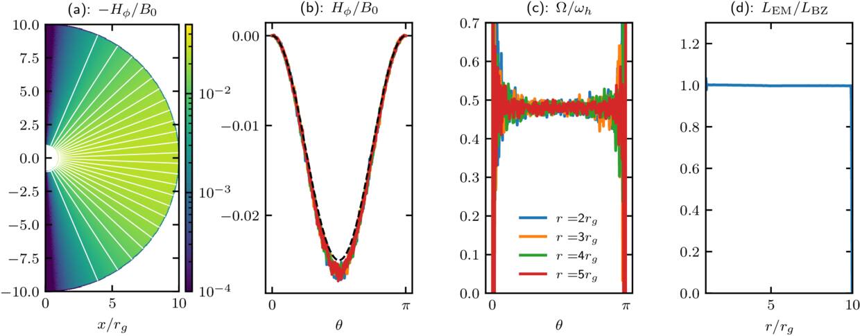
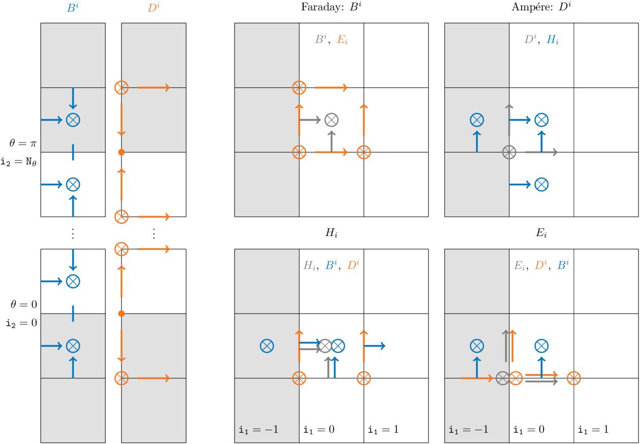
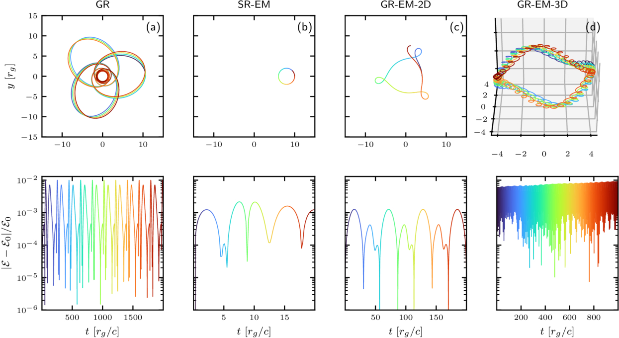
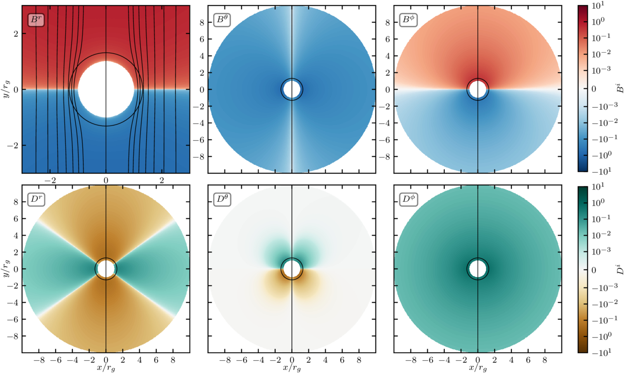
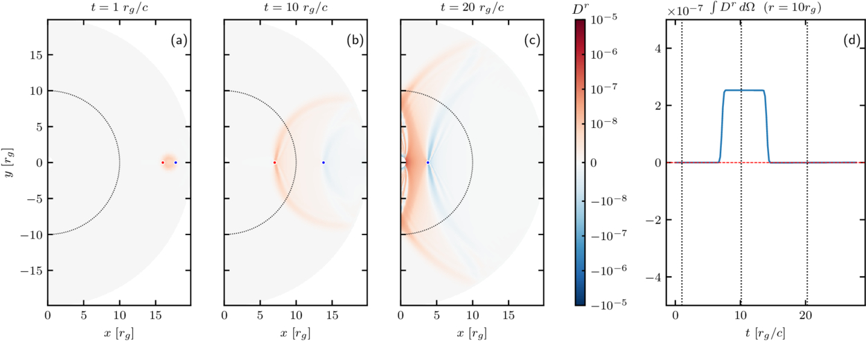
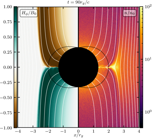
Figure 6. Snapshot of the Blandford–Znajek monopole solution in GRPIC at t = 200rg for a BH spin a = 0.2. Panel (a) shows the distribution of Hϕ/B0 across the domain, with white lines indicating magnetic field lines. Panels (b) and (c) present the θ-profiles of Hϕ/B0 and Ω/ωh, respectively, at four different radii; the analytic solution for Hϕ is shown by the black dashed line in panel (b). Panel (d) displays the electromagnetic Poynting flux as a function of radius, normalized by the Blandford–Znajek luminosity, LBZ.
Download figure:
Standard image High-resolution image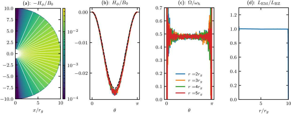
To test convergence toward the BZ solution, we compute Hϕ and compare it with the analytic monopole solution of R. D. Blandford & R. L. Znajek (1977)

at several radii (Figure 6(b)), showing good agreement between simulation results and BZ calculation.
We further compute the angular velocity of magnetic field lines as

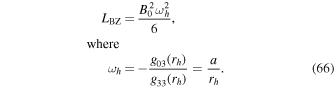
and find that it peaks at the expected value of 0.5ωh, where ωh is the BH angular frequency (given below). The departure from 0.5ωh seen in panel (c) near the poles is due to the singular behavior of  on the axis. Consequently, even small numerical fluctuations in Eθ and Br can be strongly amplified near the poles.
Finally, we evaluate the electromagnetic Poynting flux

where

and find that it roughly follows the analytic BZ luminosity (Figure 6(d))
5. Summary
In this paper, we presented the general relativistic module of the architecture-agnostic open-source PIC code Entity. The module implements a set of algorithms which integrate the trajectories of charged particles and the electromagnetic fields in the axisymmetric (2.5D) curved spacetime using the 3+1 formalism in Kerr–Schild coordinates, with an optional quasi-spherical mapping. We demonstrated a set of standard problem generators and tests, together with the relevant parameter inputs, both of which are distributed with the core of the code and are freely available.11 While the present release supports 2.5D axisymmetric Kerr–Schild coordinates, future work will extend the method to 3D using the cubed-sphere mesh.
Acknowledgments
The authors would also like to thank K. Parfrey and E. Quataert for their helpful comments and countless fruitful discussions. The initial development of the code was supported by U.S. DOE grant DE-AC02-09CH11466, NSF Cyberinfrastructure for Sustained Scientific Innovation grant 2311800, and the NVIDIA Corporation Academic Hardware Grant Program. The authors would also like to acknowledge the OLCF Director’s Discretion Project AST214 which enabled the testing of the code on the Frontier supercomputer. This work was facilitated by Simons Foundation (00001470, A.P.), and Multimessenger Plasma Physics Center (MPPC, A.P.), NSF grant No. PHY-2206607. A.P. additionally acknowledges support by an Alfred P. Sloan Fellowship, and a Packard Foundation Fellowship in Science and Engineering. The computations in this work were, in part, run at facilities supported by the Scientific Computing Core at the Flatiron Institute, a division of the Simons Foundation. The developers are pleased to acknowledge that the work was performed using the Princeton Research Computing resources at Princeton University which is a consortium of groups led by the Princeton Institute for Computational Science and Engineering (PICSciE) and Office of Information Technology’s Research Computing.
Appendix: Metric
We adopt Kerr–Schild (KS) coordinates throughout (see the project wiki at https://entity-toolkit.github.io/wiki/ for reference formulas). The expressions below provide all metric components, tetrads, and spatial derivatives required by the GRPIC particle pusher. In practice, the 3+1 split supplies the lapse, shift, and spatial metric for field evolution, while metric derivatives enter the particle pusher for accurate trajectory integration. Tetrad transformations provide a locally orthonormal frame that the pusher uses for electromagnetic fields and particle velocities.
The covariant and contravariant metrics are
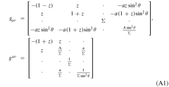
with
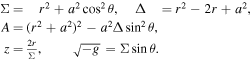
In the 3+1 decomposition, the spatial metric and its inverse are
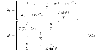
The lapse function α and shift vector βi are
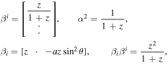
with  . Thus, specifying β1 is sufficient.
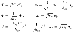
It is convenient to define a locally orthonormal tetrad basis, constructed via
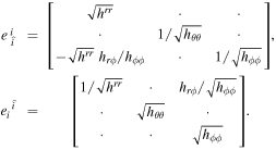
Transformations between coordinate and tetrad bases follow
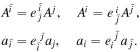
Explicitly,
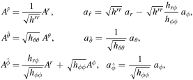
and the inverse,
Assuming general parameterization of coordinates, θ = θ(y) and r = r(x), the spatial derivatives required for the pusher algorithm are
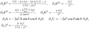
and
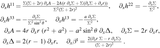
For each of the three metrics compatible with the GRPIC module in Entity, we explicitly provide the covariant and contravariant 3-metric components, tetrad transformations, and metric derivatives required for the particle pusher.
A.1. Spherical Minkowski
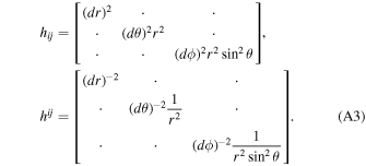
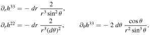
For all of our 2D simulations we adopt dϕ ≡ 1. The kerr_schild_0 metric in Entity is used primarily for testing purposes; it corresponds to a spherical grid in flat Minkowski spacetime. The spatial metric and its inverse are
The lapse and shift are trivial:

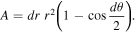
and  . The functional form of the polar area A used for the field solver is
All derivatives vanish except
A.2. Spherical Kerr–Schild
In spherical Kerr–Schild coordinates, kerr_schild, the spatial metric and its inverse are
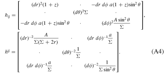
The corresponding lapse function and shift vector are

and  . The functional form of the polar area A used for the field solver is

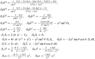
The derivatives used by the pusher are
A.3. Quasi-spherical Kerr–Schild
We also implement a quasi-spherical KS coordinate system qkerr_schild. The radial and polar coordinates are remapped as
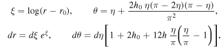
where r0 is a radial offset and h0 controls the concentration of grid points toward the equator.
All spherical KS coefficients remain valid but are now functions of (ξ, η). The spatial metric and its inverse are

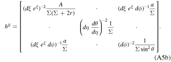
The lapse and shift are

and  . The functional form of the polar area A used for the field solver repeats the functional form of kerr_schild but expresses it through the ξ and η variables in practice.
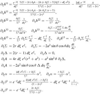
The derivatives needed by the pusher are
A.4. Transformation between BL and KS
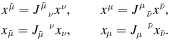
For comparison with other works and to connect with the physically more intuitive BL frame, it is useful to write down the explicit transformation between BL and KS coordinates. If gμν denotes the metric in KS coordinates and  the metric in BL coordinates, the Jacobian matrices relating the two are
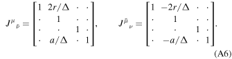
The transformations of contravariant and covariant components follow directly:
Footnotes
- 7
GitHub link: https://github.com/entity-toolkit/entity; documentation is provided at https://entity-toolkit.github.io.
- 8
The contravariant components can be obtained as ui = hijuj − u0βi, and the time component satisfies αu0 = γ.
- 9
As in the SR case, we also tested the integral form of the evolution equation for D1 on the axes. The two approaches agree at low resolution. At high resolution, however, the zero-gradient condition proves to be more stable in the case of nonzero black hole spin.
- 10
We make these distinction since most test orbits in the literature are presented in Boyer–Lindquist coordinates, while Entity operates in Kerr–Schild coordinates.
- 11
GitHub link: https://github.com/entity-toolkit/entity.