


Abstract
We present new JCMT SCUBA-2 observations of the Galactic Center region from  and
and  , covering 10 × 2 square degrees along the Galactic Plane to a depth of 43 mJy beam−1 at 850 μm and 360 mJy beam−1 at 450 μm. We describe the mapping strategy and reduction method used. We present 12CO(3-2) observations of selected regions in the field. We derive the molecular-line conversion factors (mJy beam−1 per K km s−1) at 850 and 450 μm, which are then used to obtain the amount of contamination in the continuum maps due to 12CO(3-2) emission in the 850 μm band. Toward the fields where the CO contamination has been accounted for, we present an 850 μm CO-corrected compact source catalog. Finally, we look for possible physical trends in the CO contamination with respect to column density, mass, and concentration. No trends were seen in the data despite the recognition of three contributors to CO contamination: opacity, shocks, and temperature, which would be expected to relate to physical conditions. These SCUBA-2 Galactic Center data and catalog are available via https://doi.org/10.11570/17.0009.
Export citation and abstract BibTeX RIS
1. Introduction
The center of our Galaxy provides a unique view of star and cluster formation in an extreme environment. The dominance of forces such as tidal shearing, powerful magnetic fields, and high levels of turbulence make the conditions here quite different from those found in the rest of the Galactic disk (Morris & Serabyn 1996). An understanding of these conditions and how they dictate star formation is essential to building a link between local star-forming regions and star formation in external galaxies. Molecular clouds near the Galactic Center can be divided into the Central Molecular Zone (CMZ) and high-velocity-dispersion clouds (the l = 1.3 complex; Rodriguez-Fernandez et al. 2006; Liszt 2008; Bally et al. 2010).
The CMZ is a region within a radius of ∼200 pc from the Galactic Center, and is characterized by high gas temperatures (∼80 K) and densities ( cm−3). It has been shown that 10% of the CO molecular gas in the Galaxy resides within this relatively small region (Morris & Serabyn 1996). The CMZ particularly stands out in dense gas tracers; for example, 80% of the integrated NH3(1,1) (
 cm−3) content of the Galaxy is found within the CMZ (Longmore 2012). Molecular clouds in the CMZ are found to be massive (on the order of
  , Immer et al. 2012) and dense, as smaller and/or less-dense clouds are torn apart by tidal shearing (Morris & Serabyn 1996). As a result, the CMZ contains the most-massive molecular clouds in the Milky Way, including the Sgr A and Sgr B complexes. It has been proposed recently that the well-known cloud structures and complexes of the CMZ lie along a twisted/partial-ring structure (Sawada et al. 2004; Liszt 2008; Molinari et al. 2011), with the clouds sharing a common timeline (Longmore et al. 2013; Kruijssen et al. 2015; Henshaw et al. 2016).
Although these CMZ clouds all have densities and pressures well above the threshold for star formation, the star formation rate turns out to be unusually low: there is no corresponding enhancement in the frequency of star formation tracers such as methanol masers (Caswell 1996; Immer et al. 2012), water masers (Taylor et al. 1993), or H ii regions (Bania et al. 2010). Kauffmann et al. (2013) found this region to have a factor of 45 fewer YSOs per unit volume compared with standard star-forming models (Lada et al. 2010).
The high-velocity-dispersion clouds include Bania's Clump 2 located at  (Bania 1977) and the cloud complex at
  (Bally et al. 1988). Bania's Clump 2 is an interesting complex with large line widths of ∼100 km s−1 (Riffert et al. 1997) and a large reservoir of material (
 Stark & Bania 1986), yet it has little signs of star formation (Bally et al. 2010). In velocity space Bania's Clump 2 contains a sharp feature in velocity (Liszt 2008; McClure-Griffiths et al. 2012) that has been discussed in the literature (Stark & Bania 1986; Liszt 2008; Bally et al. 2010; McClure-Griffiths et al. 2012) with a widely accepted view that this is a cloud entering a dust lane being shocked. The
  complex (Bally et al. 1988; Oka et al. 1998, 2001) is another cloud complex with a large extent in velocity, ∼100 km s−1 (Oka et al. 1998), and no signs of current star formation (Tanaka et al. 2007). This complex may have been formed from several supernova explosions, with a total mass on the order of
  (Oka et al. 2001; Tanaka et al. 2007).
Understanding the conditions surrounding star formation requires large unbiased data sets and much work has been done in the last decade to produce such data. The original SCUBA instrument at the James Clerk Maxwell Telescope (JCMT) provided the first large submillimeter map of the Galactic Center (Pierce-Price et al. 2000). In recent years there have been a number of large-scale Galactic Plane surveys, many of which include the central region. Surveys tracing continuum emission include, in order of increasing wavelength, GLIMPSE (Benjamin et al. 2003); Hi-GAL (Molinari et al. 2016); ATLASGAL (Schuller et al. 2009); and the Bolocam Galactic Plane Survey (Aguirre et al. 2011). Line surveys include HOPS (NH3, H2O, and CH3OH maser lines; Walsh et al. 2011; Purcell et al. 2012), various transitions of CO (Oka et al. 1998, 2006; Dame et al. 2001), and also the Australia Telescope Compact Array HI Survey of the Galactic Center (McClure-Griffiths et al. 2012).
We have made use of the increased mapping speed of SCUBA-2 to expand on the original SCUBA map of Pierce-Price et al. (2000). The new data presented in this paper cover a 10° × 2° strip across the Galactic Center at 450 μm and 850 μm. This data set complements other surveys and contributes to an unbiased picture of star formation in the Galactic Plane. These data will be particularly powerful when combined with the data from the SCUBA-2 JCMT Plane Survey (JPS; Moore et al. 2015). The JPS has mapped the Galactic Plane in six 6° strips at intervals between Galactic longitudes 8° and 62° using a similar mapping strategy as used in the present paper. In addition, these data will complement the high-resolution survey of the CMZ region by the Submillimeter Array known as the CMZoom survey (Battersby et al. 2016), which will collect data pertaining to both the dust continuum and spectral lines around 1.3 mm.
2. Observations and Data Reduction
2.1. SCUBA-2 Observations
SCUBA-2, the Sub-millimetre Common-User Bolometer Array-2, is a 10,000 pixel bolometer camera that images 450 μm and 850 μm simultaneously with half-power beam sizes of ∼8'' and ∼13'' respectively (Holland et al. 2013). SCUBA-2 is mounted on the left Nasmyth platform of the 15 m JCMT, located close to the summit of Maunakea, Hawaii.
The data for this 10° × 2° Galactic Center map were obtained between 2012 May and August. The region was covered by 55 partly overlapping fields observed as 25-minute circular one-degree "pongs" (Kackley et al. 2010; Holland et al. 2013). The latitudes of the fields were ± 0 41 and spaced in longitude by 039. The final map covering the region
  and
and  , can be seen in Figure 1.

Figure 1. The full SCUBA-2 850 μm coverage. Regions of brighter 850 μm emission are highlighted. These regions are also depicted in Figures 2, 3 and 5.
Download figure:
Standard image High-resolution imageThe low declination of the Galactic Center posed a challenge when trying to ensure relatively even noise in the final maps. We split the observations into three groups: fields with a low, medium, or high elevation at transit. Observing constraints were implemented so that low-elevation fields ( ) were observed in "dry" weather (
 ), medium-elevation fields were observed in "medium dry" weather (
 ), and high elevation fields (
 ) were observed in poorer weather (
 ). This observing strategy resulted in a reasonably smooth rms distribution at 850 μm.
In addition to these observations, we have also included the publicly available data taken of the Galactic Center during commissioning.5 These data, collected in 2011, differ slightly from the data collected for the project in both elapsed time and observing mode (see Table 1).
Table 1. Summary of SCUBA-2 Observations
| Program Dataa | JSA Datab | |||
|---|---|---|---|---|
| 850 μm | 450 μm | 850 μm | 450 μm | |
| no. observations | 65 | 51 | 3 | 1 |
| scan speedc (arcsec s−1) | 600 | 600 | 600 | 600 |
| scan spacingd (arcsec) | 180 | 180 | 60 | 60 |
| no. scan rotationsd | 8 | 8 | 3 | 3 |
| lengthe (minutes) | 25 | 25 | 40 | 40 |

|
<0.12 | <0.08 | <0.09 | <0.08 |
Notes.
aData obtained for the SCUBA-2 Galactic Center program presented in this paper. bData obtained from the JCMT Science Archive (Economou et al. 2015) and used in addition to the program data. cIdentical scanning speeds across all data ensure the spatial filter scales remain constant. dFor more details on scan speed and scan rotations see Holland et al. (2013). eThe elapsed time per observation.Download table as: ASCIITypeset image
Calibration observations were taken approximately five times per night to confirm the stability of the calibration to within 20% of the expected values (Dempsey et al. 2013a).
Besides the normal calibration observations, we also carried out a single calibration observation of Uranus using the same one-degree scan pattern as our Galactic Center science observation. This enabled us to investigate the effect of our observing and data-reduction method on the SCUBA-2 flux calibration in comparison with JCMT's routine calibrator observations. (see Section 2.2).
SCUBA-2 pointing observations of nearby point sources were typically done hourly. During the nights of our observations these pointings show an rms deviation of 1 6 in azimuth and 19 in elevation.
2.2. Data Reduction
The data presented in this paper were reduced with the Dynamic Iterative Map-Maker (see Chapin et al. 2013), which is available as part of the Starlink (Currie et al. 2014) SMURF package (Jenness et al. 2011, ascl:1310.007) as the command makemap. We used a "two step" process similar to the "GBS LR1" reduction method (Mairs et al. 2015) employed by the Gould Belt Survey team (Ward-Thompson et al. 2007). This method is referred to as a "two step process" because the process involves running makemap twice on the same data. The process involves (1) a reduction of each observation with an initial configuration; mosaicking these observations together and producing an emission mask from the combined map and (2) reducing each observation again, this time using the emission mask created from all the observations to constrain the flux density.
In the initial step in this process, all observations were reduced using the configuration file dimmconfig_bright_extended.6 This is the "automask" reduction step (using the terminology of Mairs et al. 2015); the emission mask used by makemap during its iterative process for each observation is created by the software using only the information in that single observation.
In the second step of the process these automasked maps were co-added, and the emission mask for the final reduction was formed. Usually, when creating an external emission mask, one chooses to threshold the data so as to only include well-detected emission (at a greater than 1σ to 3σ level). Instead, we allowed the mask to extend down to the rms noise level in the map. This was done by setting a flux masking level of 0.0 for inclusion of regions into the mask: i.e., including all regions with a signal-to-noise ratio greater than one. This method was found in JCMT internal testing to encourage the mapmaker to search for emission without artificially inflating small-scale instabilities. To complete our reduction, we then reduced the raw observations again. We used the same configuration file as above, but also incorporated our emission mask to constrain the flux (through the makemap AST model parameters ast.zero_snr and ast.zero_mask).
The 450 μm data were reduced in an identical manner to the 850 μm data, with an additional requirement that only data obtained in "dry" and "medium dry" weather ( ) were included (see Table 1). Because of the higher opacity at 450 μm the signal-to-noise ratio of these data is lower than that of the 850 μm data and maps showing only the brightest emission regions. Therefore, the 450 μm data are provided along with this paper only for completeness.
In addition to the 850 and 450 μm Galactic Center data, the corresponding one-degree Uranus observation was run though our specific reduction method. This enabled a comparison of the output from the data reduction outlined in this paper to the standard calibration. This change in reduction method led to a difference in the flux conversion factor (FCF) of less than 3% compared with the standard FCFs (537 Jy pW−1 beam−1 at 850 μm and 491 Jy pW−1 beam−1 at 450 μm; Dempsey et al. 2013a); therefore, we have chosen to apply the standard FCFs at both wavelengths.
In a final step, the individual observations of the Galactic Center were co-added. Within the central 5° by 2° area, the rms noise in the resulting 3'' pixel maps is typically 39 mJy beam−1 at 850 μm and 375 mJy beam−1 at 450 μm. Across the regions mapped in 12CO (3-2) (see Section 2.3.1), the SCUBA-2 rms noise is 35 mJy beam−1 at 850 μm and 393 mJy beam−1 at 450 μm. For comparison, the map produced by Pierce-Price et al. (2000) reached depths of 30 mJy beam−1 at 850 μm, and 300 mJy beam−1 at 450 μm. This new SCUBA-2 map expands the on-sky coverage of this region by a factor of 14. In addition, this data can also be compared to ATLASGAL, which has a depth of between 50 and 70 mJy beam−1 at 870 μm with a beam FWHM of 192 (Contreras et al. 2013). The SCUBA-2 data presented here can be obtained at the CADC space and are shown in Figures 1 and 2.

Figure 2. Three color images formed from the Herschel PACS 70 μm (taken from Molinari et al. 2016, the Hi-GAL first public data release) in red; the SCUBA-2 850 μm image in blue; and the integrated 12CO (3-2) HARP observations in green. Top: the Central Molecular Zone (CMZ). Bottom left: image of Bania's Clump 2 region. Bottom center: image of the l = 1.3 complex. Bottom right, top: the South 1 field. Bottom right, bottom: the South 2 field.
Download figure:
Standard image High-resolution image2.3. CO Contamination
Continuum observations taken by SCUBA-2 at both 450 μm and 850 μm are known to be affected by contamination from spectral lines (Johnstone et al. 2003). The dominant source of contamination at these submillimeter wavelengths is carbon monoxide. At 450 μm the center of the bandpass filter at 664 GHz is close to the 12CO(6-5) line (at 691.473 GHz). At 850 μm, the center of the bandpass filter at 347 GHz is close to the 12CO(3-2) line (at 345.796 GHz).
The importance of understanding the amount of CO contamination when determining temperature, spectral index, and dust-grain emissivity, in particular in regions of lower column density, was demonstrated by Coudé et al. (2013), Hatchell et al. (2013), and Coudé et al. (2016) in Orion A and Perseus and previously for the SCUBA (Holland et al. 1999) instrument by Johnstone et al. (2003). Such investigations have demonstrated the variation in CO contamination as a function of environment. In Orion B, toward some denser cores in the brighter regions of NGC 2023 and 2024, contamination values reach above 50% and in the NGC 2071 cluster it reaches above 20% (Kirk et al. 2016). Although considerable, these high values tend to be rare, with lower values <20% being more typical (Nutter & Ward-Thompson 2007; Buckle et al. 2015; Rumble et al. 2015).
Drabek et al. (2012) were the first to quantify the 12CO (3-2) contamination for SCUBA-2 using observations of the Perseus and Orion B regions. Looking at sources identified by Nutter & Ward-Thompson (2007) as young stellar objects, they found that the typical contamination within these sources at 850 μm was under 20%, but could increase to almost 80% in regions where molecular outflows are present. The contamination at 450 μm was reported to be negligible by comparison.
To investigate the level of CO contamination within the Galactic Center complex, targeted observations of 12CO (3-2) toward six regions of interest (12 fields in total) were made. The choice of targets was made to include bright noteworthy regions and regions with lower dispersed emission. The six regions chosen are shown in Figure 3 and detailed in Table 2.
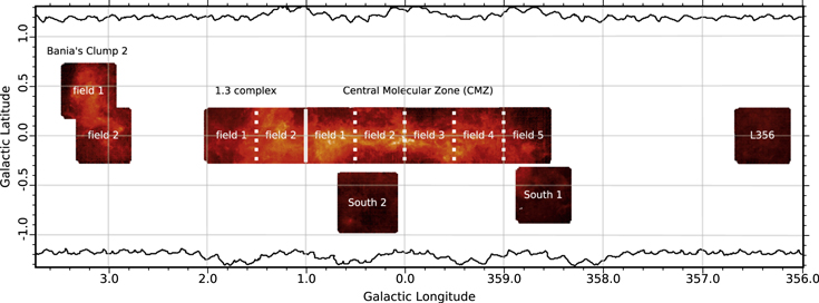
Figure 3. 12CO (3-2) integrated-intensity map with all the HARP regions and fields identified (see Table 2). The outline indicates the SCUBA-2 coverage within the region shown.
Download figure:
Standard image High-resolution imageTable 2. Summary of HARP 12CO (3-2) Observations (See Also Figure 3)
| Regiona | Fieldb | Positionc | Coverage | CCOd | Notes | |
|---|---|---|---|---|---|---|
| l (°) | b (°) | (°) | (%) | |||
| Bania's Clump 2 | 1 | 3.20 | 0.45 | 0.5 × 0.5 | 56 | High-velocity-dispersion cloud |
| 2 | 3.05 | 0.00 | 0.5 × 0.5 | 47 | High-velocity-dispersion cloud | |
| l = 1.3 Complex | 1 | 1.75 | 0.00 | 0.5 × 0.5 | 26 | High-velocity-dispersion cloud |
| 2 | 1.25 | 0.00 | 0.5 × 0.5 | 38 | High-velocity-dispersion cloud | |
| CMZ | 1 | 0.75 | 0.00 | 0.5 × 0.5 | 25 | Galactic Center |
| 2 | 0.25 | 0.00 | 0.5 × 0.5 | 40 | Galactic Center | |
| 3 | 359.75 | 0.00 | 0.5 × 0.5 | 41 | Galactic Center | |
| 4 | 359.25 | 0.00 | 0.5 × 0.5 | 44 | Galactic Center | |
| 5 | 358.75 | 0.00 | 0.5 × 0.5 | 33 | Galactic Center | |
| South 1 | ⋯ | 358.60 | −0.60 | 0.5 × 0.5 | 6 | Emission below the plane |
| South 2 | ⋯ | 0.375 | −0.68 | 0.55 × 0.55 | 7 | Emission below the plane |
| L356 | ⋯ | 356.40 | 0.00 | 0.5 × 0.5 | 5 | Low-emission region |
Notes.
aRegions are defined here as areas of contiguous HARP coverage. bEach region consists of a number of individual observations. cThe central position of each field is provided in Galactic Plane coordinates. dAverage contamination as estimated over pixels, with CO-corrected 850 μm flux .
.
Download table as: ASCIITypeset image
2.3.1. HARP Observations
The 12CO (3-2) data were obtained using HARP (Heterodyne Array Receiver Program) together with the digital auto-correlator spectrometer ACSIS (Auto-Correlation Spectral Imaging System) on the JCMT (Buckle et al. 2009). HARP has 16 SIS receptors that operate between 325 and 375 GHz, although during our observations only 12 were operational. All observations were taken using the "basket weave" (observations taken with perpendicular scan directions) raster method. HARP's receptors are arranged in a 4 × 4 array separated by 30'', with a beam size of 14'', which means the sky is under-sampled (Buckle et al. 2009). The field of view can be rotated using the "k-mirror" in the beam, specifically by rotating it to 1448 with respect to the scan direction to produce a fully sampled image (Buckle et al. 2009).
The 12 fields of the Galactic Center mapped by HARP were made up of ∼05 × 05 individual observations using scans with 1/2 array spacing. We used ACSIS with a bandwidth of 1800 MHz, which resulted in a spectral resolution of 0.97 MHz.
2.3.2. HARP Data Reduction
The heterodyne spectra from HARP were reduced with the automated astronomical reduction pipeline ORAC-DR (Jenness & Economou 2015, ascl:1310.001), using the techniques described in Jenness et al. (2015).
The chosen recipe was REDUCE_SCIENCE_GRADIENT. This sorted the time-series spectra into temporal order. Then it merged the two sub-bands by determining the offset between bands by a comparison of values in the overlap but excluding the noisy ends, typically being about thirty channels. The absolute offsets from the median differences were typically a few mK to 0.08 K. With <3% of spectra in the observations deemed to have too much high-frequency noise and excluded. For rejection of nonlinear baselines, different exclusion zones were chosen depending on the extent in velocity of the emission region. Rejection fractions for nonlinear baselines varied by observation to between 2% and 30%.
Then followed an iterative phase where the time-series cube was converted to a spectral-line cube whose coordinates were galactic and radial velocity ( ). In this cube, linear baselines were fitted and subtracted, and emission was detected and masked. As an iterative step, these masks were then applied to the original data with the aim of excluding all the emission that would bias the baseline fitting. The final step in the iteration was to apply flat-field corrections following the basic principles of Curtis et al. (2010). The summed flux determined from stronger emission regions over fixed velocity ranges included all the time series for each detector to improve the signal-to-noise ratio, but individual observations were corrected independently. The correction factors for adjacent observations in a basket weave agreed within a few percent. Then the process was repeated except for the reformed time-series cube and final created products, again only with linear baseline subtraction. The large velocity dispersion of the emission made fitting higher-order baselines problematic.
The spectral cubes have a spatial binning of 6'', and were formed with a Gaussian smoothing kernel of 9'', giving an effective resolution of 166. The original spectral resolution of 0.85 km s−1 was retained and the velocities were found with respect to the kinematical local standard of rest. The rms noise varied typically between 0.4 and 0.84 K due to variations in observing conditions.
The data were then converted to  , where we used the forward spillover and scattering efficiency
  of 0.71 to convert from
  as we examined scales larger than the beam size.
The HARP data are shown in Figure 2 along with the SCUBA-2 850 μm emission. An integrated-intensity image (−215–220 km s−1) of the HARP data is given in Figure 3 with the 12 fields identified, and a summary of the data is given in Table 2.
2.3.3. Estimating the Contamination: The Method
To estimate the level of CO contamination in the SCUBA-2 fields, we subtracted HARP 12CO (3-2) emission from the raw SCUBA-2 time-series data during the initial steps of the makemap reduction process, following Hatchell et al. (2013) and Sadavoy et al. (2013). The SCUBA-2 CO-subtracted raw data were then used for both steps of the SCUBA-2 reduction process: the initial reduction and the external emission-mask reduction (as outlined in Section 2.2). The original SCUBA-2 map was then compared with the SCUBA-2 CO-subtracted map over the regions containing HARP data. Differences between these maps were then attributed to the contamination by the CO line at 345.796 GHz. The benefit of this method (subtracting the 12CO emission before the reduction process), is that the same spatial filtering is applied to both data sets.
2.3.4. CO-line Conversion Factor
To utilize the HARP 12CO(3-2) data in the SCUBA-2 reduction, the HARP data had to first be converted from  to mJy and then to pW, the units used for raw SCUBA-2 data. We followed the method outlined by Drabek et al. (2012) to produce the molecular-line conversion factor at 850 μm, C850, in terms of precipitable water vapor (PWV) in millimeters (mm), with a few key differences:
- 1.We fitted a fourth-order Lagrange polynomial to the values quoted in Table 1 of Drabek et al. (2012) in order to yield the conversion factor C850 (mJy beam−1 per K km s−1), as a function of opacity at 225 GHz (
 ).
). - 2.The fit uses an updated main-beam FHWM of 130 at 850 μm, with a relative amplitude of 0.98 (Dempsey et al. 2013a).
- 3.The fit includes a correction for the secondary beam component, as we are interested in structures that are bright and extended. The secondary beam component is 480, with a relative amplitude of 0.02 (Dempsey et al. 2013a).

Describing the conversion factor as a function of PWV is required due to the SCUBA-2 filter profiles changing as a function of PWV (for more information see Figures 1 and 2 in Drabek et al. 2012). This conversion factor is expressed as:
where the values α, β, γ, δ, and  are listed in Table 3 for both C850 and C450 (the 450 μm relationship).
Table 3. List of Coefficients for Use in Determining the Conversion Factor C850 and C450 as Described in Equation (1)
| Coefficient | 850 μm | 450 μm |
|---|---|---|
| α | 0.574 | 0.761 |
| β | 0.1151 | 0.0193 |
| γ | 0.0485 | 0.0506 |
| δ | 0.0109 | 0.0141 |
|
0.000856 | 0.00125 |
Download table as: ASCIITypeset image
The coefficients for the C450 relationship are provided for completeness in Table 3. These values were determined in an identical manner to those for C850, but we note that at 450 μm the main-beam FWHM is 79, with a relative amplitude of 0.94, a secondary beam FWHM component of 25'', and a relative amplitude of 0.06 (Dempsey et al. 2013a).
Equation (1) is expressed in terms of PWV, which is related to the sky opacity at 225 GHz,  as (Dempsey et al. 2013a):

The uncertainties in the above equations depend on the accuracy of the SCUBA-2 filter shapes and the accuracy of the atmospheric model. A true estimate of the error is difficult to produce but is unlikely to exceed 20% and is probably dominated by uncertainties in the HARP and SCUBA-2 calibrations (Buckle et al. 2009; Drabek et al. 2012; Dempsey et al. 2013a). A comparison of these new functions and the values quoted by Drabek et al. (2012) is given in Figure 4.

Figure 4. C factor as a function of PWV. Top: 450 μm. Bottom: 850 μm. The solid lines are the fit as outlined in this paper. The data points plotted are the original C factor values as reported by Drabek et al. (2012) for comparison. The shaded region in the C450 plot denotes the ±10% level, and the shaded region in the C850 plot denotes the ±5% level.
Download figure:
Standard image High-resolution imageThe conversion factor converts the HARP data from  to mJy beam−1. As a final step the converted HARP data are divided by the FCF to obtain the HARP data in terms of pW units.
2.3.5. Contamination Results
The median CO contamination percentage is given for each field in Table 2 and varies by an order of magnitude across the regions. We provide CO contamination estimates for each compact source in Table 4 (see Section 3), and CO contamination plots for the regions are given in Figure 5. We find that the levels of CO contamination within our 850 μm maps are of the order of 35%.
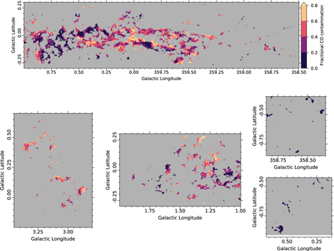
Figure 5. CO-contamination fraction from 0% to 80%. Top: CMZ. Bottom left: Bania's Clump 2 region. Bottom middle: l = 1.3 complex. Bottom left, top: the South 1 field. Bottom left, bottom: the South 2 field.
Download figure:
Standard image High-resolution imageTable 4. The First 20 of 2362 Sources from the SCUBA-2 Galactic Center 850 μm CO-corrected Compact Source Catalog
| Name | lmax | bmax | l | b | Reff | Speak | Δ Speak | Sint | Δ Sint | S/N | C | CCO |
|---|---|---|---|---|---|---|---|---|---|---|---|---|
| (°) | (°) | (°) | (°) | ('') | (Jy beam−1) | (Jy beam−1) | (Jy) | (Jy) | ||||
| (1) | (2) | (3) | (4) | (5) | (6) | (7) | (8) | (9) | (10) | (11) | (12) | (13) |
| G000.004-00.025 | 0.004 | −0.025 | 359.999 | −0.025 | 43 | 1.11 | 0.04 | 8.15 | 0.06 | 30.3 | 0.70 | 67 |
| G000.006+00.156 | 0.006 | 0.156 | 0.005 | 0.157 | 59 | 1.20 | 0.04 | 7.73 | 0.11 | 33.7 | 0.86 | 20 |
| G000.006+00.048 | 0.006 | 0.048 | 0.005 | 0.049 | 24 | 0.33 | 0.03 | 1.29 | 0.01 | 10.1 | 0.48 | 73 |
| G000.007+00.274 | 0.007 | 0.274 | 0.005 | 0.272 | 42 | 0.26 | 0.05 | 2.44 | 0.11 | 5.3 | 0.60 | ⋯ |
| G000.007+00.114 | 0.007 | 0.114 | 0.009 | 0.120 | 34 | 0.41 | 0.03 | 2.68 | 0.03 | 11.9 | 0.55 | 28 |
| G000.007+00.091 | 0.007 | 0.091 | 0.007 | 0.093 | 23 | 0.24 | 0.03 | 0.64 | 0.01 | 7.2 | 0.61 | 63 |
| G000.009+00.059 | 0.009 | 0.059 | 0.013 | 0.066 | 33 | 0.34 | 0.03 | 1.85 | 0.03 | 10.4 | 0.62 | 54 |
| G000.011-00.258 | 0.011 | −0.258 | 0.006 | −0.262 | 14 | 0.21 | 0.04 | 0.24 | 0.01 | 5.8 | 0.53 | ⋯ |
| G000.014+00.020 | 0.014 | 0.020 | 0.008 | 0.020 | 31 | 0.52 | 0.03 | 3.17 | 0.03 | 15.0 | 0.53 | 61 |
| G000.014-00.020 | 0.014 | −0.020 | 0.015 | −0.016 | 55 | 1.60 | 0.04 | 16.79 | 0.09 | 44.3 | 0.73 | 66 |
| G000.014-00.052 | 0.014 | −0.052 | 0.010 | −0.056 | 41 | 1.39 | 0.04 | 10.34 | 0.05 | 39.3 | 0.67 | 52 |
| G000.017+00.036 | 0.017 | 0.036 | 0.016 | 0.036 | 49 | 1.13 | 0.03 | 10.63 | 0.06 | 33.2 | 0.70 | 64 |
| G000.021+00.003 | 0.021 | 0.003 | 0.018 | 0.006 | 46 | 0.75 | 0.03 | 6.87 | 0.06 | 22.5 | 0.66 | 53 |
| G000.021-00.052 | 0.021 | −0.052 | 0.021 | −0.051 | 35 | 1.61 | 0.04 | 6.97 | 0.04 | 42.8 | 0.73 | 56 |
| G000.022+00.156 | 0.022 | 0.156 | 0.022 | 0.157 | 26 | 0.45 | 0.04 | 1.31 | 0.02 | 12.2 | 0.67 | 33 |
| G000.022+00.118 | 0.022 | 0.118 | 0.021 | 0.118 | 19 | 0.29 | 0.04 | 0.57 | 0.01 | 7.6 | 0.57 | ⋯ |
| G000.028-00.218 | 0.028 | −0.218 | 0.027 | −0.218 | 20 | 0.24 | 0.04 | 0.56 | 0.01 | 5.7 | 0.54 | ⋯ |
| G000.032+00.111 | 0.032 | 0.111 | 0.032 | 0.109 | 22 | 0.35 | 0.03 | 1.11 | 0.02 | 10.0 | 0.51 | 42 |
| G000.032+00.093 | 0.032 | 0.093 | 0.033 | 0.098 | 17 | 0.38 | 0.04 | 0.56 | 0.01 | 10.6 | 0.60 | ⋯ |
| G000.032+00.051 | 0.032 | 0.051 | 0.030 | 0.054 | 33 | 0.76 | 0.03 | 3.21 | 0.03 | 22.2 | 0.71 | 51 |
Note. The catalog is ordered by longitude. The columns are (1) name derived from galactic coordinates of the maximum intensity of the source; (2)–(3) galactic coordinates of the maximum intensity of the source; (4)–(5) galactic coordinates of the center intensity of the source; (6) effective source radius ( ), where A is the area of the source above the 3σ threshold; (7)–(10) peak and integrated flux densities and associated uncertainties; (11) signal-to-noise ratio (S/N); (12) concentration; (13) CO contamination.
Only a portion of this table is shown here to demonstrate its form and content. A machine-readable version of the full table is available.
Download table as: DataTypeset image
From examining Figure 5 we find that toward the Galactic Center strip (the CMZ and l = 1.3 Complex) we see a wide range in CO contamination from 0% to 80%. We see dramatic changes in contamination across the region, with the contamination appearing to be coherent on smaller scales. Within the bright (at 850 μm) structures, i.e., Sgr B1, Sgr B2, M0.25+0.01/the Brick, Sgr A*, Sgr C, G1.6-0.025, and Sgr D, we see little to no CO contamination.
This visual relation of low CO contamination with known bright structures is in contrast to what is seen in Bania's Clump 2 Complex (Bania 1977). Within this complex we find that the bright emission has CO contamination values that are, on average, higher than those in the Galactic Center (∼50%).
Away from the Galactic Center and toward regions where the sources are predominantly discrete (South 1, South 2, and L356) we find little CO contamination (values typically much less than 10%). We discuss the contamination and examine possible physical relations further in Section 4.
3. Compact Source Catalog
A compact source catalog is provided for the 850 μm data that had accompanying HARP data available for CO contamination correction (see Figure 2.3.1). A sample of this catalog is provided in Table 4 (the complete catalog is provided in the online material accompanying this paper). The compact source catalog was created using the starlink CUPID package's command findclumps with the FELLWALKER source extraction algorithm (Berry et al. 2007; Berry 2015).
The chosen source extraction method used in this paper follows the work by Moore et al. (2015) and Eden et al. (2017). As with Moore et al. (2015), Rigby et al. (2016), and Eden et al. (2017) we use the signal-to-noise map of our 850 μm CO-corrected data to produce our initial catalog. At this stage we require emission to lie above a threshold of 3σ (for the full FELLWALKER parameter list used see Appendix D of Eden et al. 2017). We additionally removed sources with peaks  and note that after this clip no sources remained with high aspect ratios (in Eden et al. 2017, data were removed if the ratio of the major to minor axis size was greater than 5.0).
CUPID's extractclumps software was used to extract these clumps from the calibrated CO-corrected data to produce the final Galactic Center CO-corrected SCUBA-2 source catalog. This final catalog contains a total of 2362 clumps (see Table 4). In this catalog, variable aperture sizes used by FellWalker to obtain integrated flux densities were accounted for using the aperture correction factors published by Dempsey et al. (2013a). To calculate the correct aperture correction factor, and following the same method of Moore et al. (2015), we compute the effective radius ( , where A is the area of the clump above the FellWalker threshold). We then use this to calculate the aperture correction factor using a fifth-order polynomial fit to the values provided by Dempsey et al. (2013a).
3.1. ATLASGAL Comparison
To check for the reliability of the compact CO-corrected source catalog data, the SCUBA-2 850 μm detections were compared to ATLASGAL 870 μm data (Schuller et al. 2009). This reliability check is consistent with that presented previously by the JPS team (see Moore et al. 2015 and Eden et al. 2017). To check for reliability, the position of the peak position from the compact source catalog (as presented in Table 4) and the peak position from the ATLASGAL catalog were matched to within a radius of 19'' (equivalent to the APEX 870 μm beam). In this way a total of 791 matches were identified.
A comparison of the SCUBA-2 peak and integrated flux densities, with respect to ATLASGAL, can be seen in Figures 6 and 7. As with Moore et al. (2015) and Eden et al. (2017), lower peak flux densities were recovered at 850 μm when compared to ATLASGAL. For consistency, a second source extraction was run on the SCUBA-2 data after convolving the 850 μm data to the APEX beam at 870 μm. When convolving to the APEX beam there is greater agreement between the 850 and 870 μm data, as seen in Figure 6. This agreement gives confidence to the reliability of the SCUBA-2 data—as also demonstrated by Moore et al. (2015) and Eden et al. (2017), who noted that this is "despite being observed with different telescopes and detectors and using unrelated techniques, reduced using different procedures and the source extraction being done using independent methods."
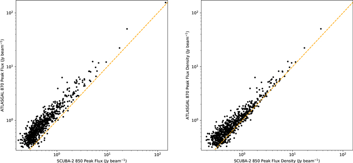
Figure 6. Comparison of the SCUBA-2 850 μm and ATLASGAL 870 μm peak flux densities (left) and 850 μm flux densities convolved to the APEX beam with the ATLASGAL 870 μm peak flux densities (right). The orange dashed line indicates the 1:1 line.
Download figure:
Standard image High-resolution image
Figure 7. Comparison of the SCUBA-2 integrated flux densities with the ATLASGAL 870 μm flux densities. The orange dashed line indicates the 1:1 line.
Download figure:
Standard image High-resolution image4. Discussion
4.1. Contamination
Any level of CO contamination can affect dust temperature and dust-grain emissivity estimates (Johnstone et al. 2003; Coudé et al. 2013; Hatchell et al. 2013 and Coudé et al. 2016), so it is a crucial consideration for any physical interpretation of data at such wavelengths.
Figure 8 provides a histogram of the distribution of CO contamination for the compact sources identified within this work. This histogram, along with Figure 5, shows how contamination by the 12CO (3-2) line can vary across a range of environments. Even in the most benign regions, such as the L356 region, CO contributes on the order of 5% to the continuum emission in the 850 μm band.

Figure 8. Distribution of CO contamination values produced for each of the compact sources identified in Section 3.
Download figure:
Standard image High-resolution imageWhen looking in more detail at the structures associated with and without substantial levels of CO contamination (>20%), it is possible to identify three key environmental mechanisms that contribute to the variations observed.
The first mechanism is the opacity of the gas. Optically thick gas failing to trace the full region (as traced by the dust) islikely the cause of low contamination values within the the Galactic Center strip toward massive clouds such as Sgr B1, Sgr B2, M0.25+0.01/the Brick, Sgr A*, and Sgr C. Moore et al. (2015) noted this in reverse—stating that higher levels of contamination were found toward the edges of continuum sources where the CO optical depth is likely to be smallest.
The second mechanism is shocks exciting the gas, leading to higher contamination values. Bania's Clump 2 complex is known to be associated with shocks (Huettemeister et al. 1998), likely due to the cloud entering a dust lane (Liszt 2008). Within this region we see higher CO contamination values (values around 50%) than those in the Galactic Center. Shocks associated with the known supernovae shells present in the l = 1.3 complex (Huettemeister et al. 1998; Oka et al. 2001) are also likely to have caused the higher CO contamination levels within this region. If we consider the median contamination between l = 1.2 and l = 1.5, we find that the contamination of this region is 44%.
The third mechanism is temperature; low temperatures found within isolated regions such as South 1, South 2, and L356 are likely to explain the minimal CO contamination in these regions. In contrast, higher temperatures may lead to lower contamination values as CO molecules become excited to higher transition levels if the gas and dust are decoupled.
These three contributions have been reported previously. Shocks have been cited as the cause of the higher contamination levels seen in Orion—up to 50% (Drabek et al. 2012; Coudé et al. 2013; Kirk et al. 2016), and higher in some instances above the typical <20% level—likely a combination of the opacity and temperature effects—observed in many regions (Nutter & Ward-Thompson 2007; Buckle et al. 2015; Rumble et al. 2015).
These three mechanisms—opacity, shocks, temperature—imply that we may be able to draw a relation between contamination and physical conditions within the Galactic Center region; we consider this further in the following section.
Correcting for the CO contamination is not only important when studying our own Galaxy but also when studying other galaxies. The Milky Way'sGalactic Center is often cited as a link between well-resolved star formation and star formation at different scales (both physical and spatial).
At distances to nearby galaxies, the HARP beam at 345 GHz is sensitive to scales around 730 pc (taking an approximate distance of 10 Mpc). For comparison, each half-degree field presented in Table 2, at a distance of 8 kpc Ghez et al. (2008) corresponds to a field of 70 pc, with the HARP central strip (the l = 1.3 complex and the CMZ) corresponding to 500 pc. At such spatial scales it should be possible to detect changes in CO contamination at 850 μm across large structures of nearby galaxies.
Indeed, Vlahakis et al. (2013) studied CO contamination in the nearby galaxy M51 (NGC 5194). The almost face-on nature of this galaxy, along with its proximity (8.2 Mpc, Tully 1974), enables the determination of such contamination across this grand-design spiral galaxy. Vlahakis et al. (2013) reports inter-arm region and outer spiral-arm contamination values of <10% (similar to our low-emission regions), 10%–20% in the spiral arms, and 20% in the central region (within a radius of 2 kpc), with a maximum of 26%.
Preliminary results from the JCMT Nearby Galaxies Survey, using CO data obtained by HARP (e.g., Wilson et al. 2009; Warren et al. 2010 etc.), have also found variations in CO contamination levels across a number of individual nearby galaxies. C.D. Wilson et al. (2017, in preparation) found typical CO contamination values of the order of 25%, with variations from 6% to 40% across a sample of 20 nearby galaxies. M51 was also included in the sample and contamination values were in agreement with the values published by Vlahakis et al. (2013).
4.2. Contamination Comparisons
To consider the CO contamination and its relation to physical conditions the median CO contamination within each source was estimated (where an estimate was available). Of the 2,362 sources CO contamination estimates are produced for 1,694 of these. The compact sources for which CO contamination estimates are available are biased to the larger brighter 850 μm sources. Note that the sources with CO contamination estimates have a median integrated intensity of 2.57 Jy and effective radius of 34'' compared to those without CO contamination estimates that have a median integrated intensity of 0.63 Jy and effective radius of 21''.
To investigate physical correlations, back-of-the-envelope estimations were made for mass, density, and source concentration. The mass and column density estimates were made by assuming that all sources lie at a distance, D, of 8 kpc (i.e., Ghez et al. 2008). In addition, a fiducial temperature, T, of 20K (i.e., Sodroski et al. 1994; Rodríguez-Fernández et al. 2004), was used. With these assumptions, mass can be estimated for each of the compact sources using the equation by Hildebrand (1983):
 is the flux density. which is reported in Table 4.
  is the Planck function.
  is the dust mass opacity (Beckwith et al. 1990),

for which we use a dust emissivity β of 2.0. From these two equations we can then estimate the mean column density using
where μ is the mean molecular weight of the gas (μ is 2.86, assuming that the gas is 70% H2 by mass, i.e., Kirk et al. 2013), mH is the mass of hydrogen, and Reff is the effective source radius (as defined and reported in Table 4). A quick examination by eye of the mass and column density estimates as a function of CO contamination—as see in Figure 9—reveals no trend. A fuller investigation, which is beyond the scope of this paper, with better temperature and distance estimates, will be required to confirm this.

Figure 9. Comparison of the CO contamination as a function of mass (left) and as a function of column density (right).
Download figure:
Standard image High-resolution imageCompactness—a metric used to quantify if the structure of a source is centrally peaked—can be estimated following the techniques by Johnstone et al. (2001). Johnstone et al. compares the total flux density across a source with the uniform structure of equivalent size but of maximum brightness (as has been implemented by Mairs et al. 2016; Kirk et al. 2017 and others). The compactness quantity, C, is calculated as follows:
where B is the beam width in arcseconds, and  is the peak flux density also reported in Table 4. The compactness quantity is provided in Table 4. An examination of the concentration quantity compared to the CO contamination for the compact sources indicates there is no obvious correlation, as seen in Figure 10.

Figure 10. Comparison of the CO contamination as a function of concentration. The vertical lines indicate the minimum concentration for a constant density low-mass Bonnor–Ebert sphere (C = 0.33), and the maximum concentration beyond which collapse occurs (C = 0.72, see Johnstone et al. 2001).
Download figure:
Standard image High-resolution image
Finally, it is possible to use the 70 μm data from the Photodetector Array Camera and Spectrometer (PACS; Poglitsch et al. 2010) from the Herschel Space Observatory to look for correlations in CO contamination with respect to the warm dust emission from protostellar sources—and as a proxy for environment. Looking at Figure 2 and the brightness of the 70 μm emission as taken from Hi-GAL (the Herschel infrared Galactic Plane Survey Molinari et al. 2016), it is difficult to see any real trends. By comparing each of the compact sources associated with a value for the CO contamination (see Table 4) with the median PACS 70 μm emission, we find no obvious correlation.
4.3. Contamination by Free–Free Emission
Alongside CO(3-2) and its impact on the 850 μm dust emission observed in both Galactic and extra-galactic environments, works by Motte et al. (2003), Schuller et al. (2009), Rumble et al. (2015), and Rumble et al. (2016) have demonstrated a second source of contribution in both the 450 and 850 μm bands: free–free emission. Most notably, these works have demonstrated contamination by free–free emission originating from ultra-compact (UC) H ii regions. Essentially, a turnover in the spectral-energy distribution shape of an UCHII region "short-ward of the submillimeter regime has a major contribution to [the] 850 μm band and [a] significant [contribution] to [the] 450 μm band" (Rumble et al. 2015).
An investigation toward the Serpens MWC 297 region, part of the larger Serpens-Aquila star-forming complex by Rumble et al. (2015), reported that free–free emission from an UCHII region accounts for 73% of the emission at 450 μm and 83% of the emission at 850 μm. Combined with the 13% CO contamination, they found that in this low-mass star-forming region, only 5% of the peak emission at 850 μm is from dust—the rest is from emission from UCHIIs and the gas.
A study of W40 by Rumble et al. (2016) found free–free emission from an associated UCHII region contributing 12% at 850 μm and 9% at 450 μm. Additional contamination from an H ii region (powered by a Herbig AeBe) star was noted, but this contamination was to a lesser extent (5% at 850 μm and 0.5% at 450 μm).
The Galactic Center, which contains a rich diverse environment for massive-star formation, is known to contain numerous UCHII regions (i.e., Wood & Churchwell 1989; Becker et al. 1994; Giveon et al. 2005; Anderson et al. 2014). It is clear that these UCHIIs could provide a significant additional contribution to the contamination in the SCUBA-2 data.
Giveon et al. (2005) identified approximately 200 UCHIIs located within the region mapped by SCUBA-2. The locations of these UCHIIs follow the well-known regions, and typically these regions are where we find lower (<5%) CO contamination. To the east of the CMZ there is Sgr B2 (De Pree et al. 1998, 2005; Etxaluze et al. 2013; De Pree et al. 2014), and G1.13-0.12 Olmi & Cesaroni (1999). Here in Sgr B2 is the largest population of UCHII regions within a single region, so emission from the dust is likely to follow the example of Rumble et al. (2016) and only account for a fraction of the emission in the 450 μm and 850 μm bands.
In the center of the CMZ, UCHII regions are located in the Arches Cluster (Bik et al. 2005), and embedded in the western ridge of M-0.02â–0.07 (Mills et al. 2011). To the west of the CMZ Sgr C there is also known to be an associated UCHII region (Kendrew et al. 2013).
South of the Galactic Center, in the South 2 Region, lies the nearby star-forming cloud G0.55-0.85 (seen in the bottom left of Figure 2). Although CO contamination is low toward G0.55-0.85 (Figure 5), the association with an UCHII may indicate that in this particular isolated region this additional contamination from free–free emission must also be considered (Gennaro et al. 2012).
Although the free–free emission from UCHII regions has a potentially significant contribution to the submillimeter continuum emission in specific star-forming regions found throughout the Galactic Center, the authors note that the locations of these contributions to emission in the 450 μm and 850 μm bands are discrete and non-uniform across the field mapped by SCUBA-2. With a distinct lack of star-forming indicators within Bania's Clump 2, it is unlikely to suffer contamination from this free–free emission. Note that there is far less PACS 70 μm emission toward Bania's Clump 2 complex and the G1.6-0.035 region in the l = 1.3 complex (see Figure 2). Using the PACS 70 μm emission as an indicator of the possible regions of young star formation, and thus the locations of objects contributing to such free–free emission, we can be confident in the flux values reported in our compact source catalog, where we see little to no PACS emission.
5. Summary
In this paper we present an updated look at the Galactic Center by the SCUBA-2 camera covering a region of 10° × 2° along the Galactic Plane. We reach a median depth of 39 mJy beam−1 at 850 μm and a depth of 375 mJy beam−1 at 450 μm. The SCUBA-2 data, along with complementary 12CO(3-2) data taken by HARP, and the produced contamination maps, are publicly available.7
This paper provides a detailed overview of the molecular-line conversion factors (mJy beam−1 per K km s−1) at 850 μm (C850) and 450 μm (C450). From this C850 conversion factor, and using HARP 12CO (3-2) data, we present the contamination on the 850 μm dust emission from this molecular gas. Toward regions where the CO contamination is accounted for, we provide an 850 μm compact source catalog containing 2363 sources. This catalog provides positional information, an effective radius, peak flux, integrated flux, concentration, and—where available—the median CO contamination within each source.
We find that contamination as traced by 12CO (3-2) has an effect at the 35% level in regions with substantial emission (close to the Galactic Center and toward Bania's Clump 2) and little to no CO contamination in discrete regions. Variation in the range of CO contamination is reflected within other galactic (Nutter & Ward-Thompson 2007; Drabek et al. 2012; Coudé et al. 2013; Buckle et al. 2015; Rumble et al. 2015; Kirk et al. 2016) and extra-galactic studies (Tully 1974; C.D. Wilson et al. 2017, in preparation).
We discussed three mechanisms controlling the level of CO contamination in the various region—opacity, shocks, temperature. Further examination of the CO contamination, against estimates of compact source masses, column densities, and source concentration, were made. No correlations were found in the data, but these physical estimates were very much "back-of-the-envelope" calculations. By eye, the CO contamination does not look random, with changes seen between structures within the CMZ and little to no contamination in the less bright, more isolated regions—such as South 1, South 2 and L356. With additional information such as distance and temperatures, a connection between the contamination and the physical conditions of a region may yet be revealed.
This contamination of submillimeter dust emission must (along with free–free emission) be considered before meaningful properties can be derived from the data.
When studying the dust emission at these wavelengths, having supplemental data to estimate contamination in the bandpass is desirable. COHRS, the CO High-Resolution Survey (Dempsey et al. 2013b), which maps a strip of the inner Galactic plane in 12CO(3-2), is an ideal resource for Galactic astronomers. The current release by Dempsey et al. (2013b) covers  between
  and
and  , and
, and  between
  . When complete, COHRS will provide coverage between
  and
and  . One prime example for the use of this data is the estimation of the CO contamination within the recently released ATLASGAL (The APEX Telescope Large area survey of the galaxy at 870 μm) data (Schuller et al. 2009). The Large APEX Bolometer Camera (LABOCA) is a 295-element bolometer array observing at 870 μm, with a beam size of 19'' (Siringo et al. 2009). As with SCUBA-2, LABOCA's filters place the strong CO(3-2) line within the instrument's bandpass and should be considered when using such data.
The James Clerk Maxwell Telescope is operated by the East Asian Observatory on behalf of The National Astronomical Observatory of Japan, Academia Sinica Institute of Astronomy and Astrophysics, the Korea Astronomy and Space Science Institute, the National Astronomical Observatories of China and the Chinese Academy of Sciences (grant No. XDB09000000), with additional funding support from the Science and Technology Facilities Council of the United Kingdom and participating universities in the United Kingdom and Canada. The program ID is M15AI72.
The James Clerk Maxwell Telescope has historically been operated by the Joint Astronomy Centre on behalf of the Science and Technology Facilities Council of the United Kingdom, the National Research Council of Canada and the Netherlands Organisation for Scientific Research. Additional funds for the construction of SCUBA-2 were provided by the Canada Foundation for Innovation. The program IDs of this project are M12AJ01, M13AD07, M13BD01, and M14AD01.
This research used the facilities of the Canadian Astronomy Data Centre operated by the National Research Council of Canada with the support of the Canadian Space Agency. This research made use of Astropy, a community-developed core Python package for Astronomy (Astropy Collaboration et al. 2013).
The authors thank Dr Mark Thompson for help with the tiling strategy used in this project. In addition, the authors thank Dr. Jane Buckle for various discussions regarding data reduction practices, Dr. Doug Johnstone and Dr. Christine Wilson for discussions regarding CO contamination, and Steve Mairs for helpful input. The authors also wish to thank the referee for the assistance and patience, which greatly improved this work.
Finally, the authors wish to recognize and acknowledge the very significant cultural role and reverence that the summit of Maunakea has always had within the indigenous Hawaiian community. We are most fortunate to have the opportunity to conduct observations from this mountain.
Facility: JCMT - James Clerk Maxwell Telescope (SCUBA-2, HARP).
Software: Starlink (Currie et al. 2014), SMURF, KAPPA, ORAC-DR, Astropy (Astropy Collaboration et al. 2013).
Footnotes
- 5
Commissioning data taken by SCUBA-2 were released to the community in 2013 January and can be found in the JCMT Science Archive at CADC: http://www.cadc-ccda.hia-iha.nrc-cnrc.gc.ca/en/jcmt/.
- 6
For the exact parameters used by dimmconfig_bright_extended see Starlink Version 2015A: share/smurf/dimmconfig_bright_extended.lis. For more information see the SCUBA-2 Cookbook SC/21 at http://starlink.eao.hawaii.edu/docs/sc21.htx/sc21.html.
- 7