


Abstract
In order to explore how the ubiquitous short-term stochastic variability in the photometric observations of Wolf–Rayet (WR) stars is related to various stellar characteristics, we examined a sample of 50 Galactic WR stars using 122 lightcurves obtained by the BRIght Target Explorer-Constellation, Transiting Exoplanet Survey Satellite and Microvariability and Oscillations of Stars satellites. We found that the periodograms resulting from a discrete Fourier transform of all our detrended lightcurves are characterized by a forest of random peaks showing an increase in power starting from ∼0.5 day−1 down to ∼0.1 day−1. After fitting the periodograms with a semi-Lorentzian function representing a combination of white and red noise, we investigated possible correlations between the fitted parameters and various stellar and wind characteristics. Seven correlations were observed, the strongest and only significant one being between the amplitude of variability, α0, observed for hydrogen-free WR stars, while WNh stars exhibit correlations between α0 and the stellar temperature, T*, and also between the characteristic frequency of the variations, νchar, and both T* and v∞. We report that stars observed more than once show significantly different variability parameters, indicating an epoch-dependent measurement. We also find that the observed characteristic frequencies for the variations generally lie between  , and that the values of the steepness of the amplitude spectrum are typically found in the range
  . We discuss various physical processes that can lead to this correlation.
Export citation and abstract BibTeX RIS

Original content from this work may be used under the terms of the Creative Commons Attribution 4.0 licence. Any further distribution of this work must maintain attribution to the author(s) and the title of the work, journal citation and DOI.
1. Introduction
Massive stars are known to show photometric and spectroscopic variability, from either intrinsic (e.g., pulsational or rotational modulation) or extrinsic (e.g., binary) sources (see e.g., Degroote et al. 2009; Blomme et al. 2011; Burssens et al. 2020). In the last few decades, with the increasing availability of space-borne observing capabilities and the development of asteroseismology, a growing number of investigations on their internal and external (i.e., wind) structures have been conducted (see e.g., Bowman 2020)
Hot, massive stars have strong radiatively driven winds. Their driving is facilitated by the transfer of the momentum of photons to the wind through the absorption or scattering by multiple spectral lines (Lucy & Solomon 1970). The dependence of the driving on the velocity gradient can lead to instabilities, as has been suggested by Lucy & White (1980) and shown numerically by Owocki et al. (1988). This process, referred to as the line deshadowing instability (LDI), leads to the formation of density inhomogeneities and perturbations in the wind-velocity structure and, as a consequence, the winds of massive, hot stars are highly clumped. More recent two-dimensional numerical simulations of typical O-type winds by Sundqvist & Owocki (2013) and Sundqvist et al. (2018) have shown that complex density and velocity structures naturally form very close to the base of stellar outflows as a consequence of the LDI, and that these are embedded in much larger low-density regions. Their results for rotating stars show that the same small-scale clumps form, but that they are now embedded in larger columns of ascending matter extending down to the base of the wind. These columns are actually corotating interaction regions (CIRs), suggesting that rotating LDI models could lead to the combination of small- and large-scale structures, which could explain both the observed stochastic and quasiperiodic spectroscopic variability in the optical emission lines (e.g., Heii λ 4686 Å) and the observed discrete absorption components (DACs) in the UV P Cygni absorption components.
The presence in the winds of these density and velocity inhomogeneities is very appealing to explain the stochastic variability observed in photometry, polarimetry, and spectroscopy. For example, Ramiaramanantsoa et al. (2019) have shown that it is possible to reproduce the observed characteristics of the nonperiodically, strongly variable BRIght Target Explorer (BRITE) optical lightcurve of the single WN8h star WR40 by including in the wind a distribution of clumps (either a power law or of all equal sizes) that Thomson scatter the continuum light from the optical photosphere.
This clumpy nature of hot, massive star winds could also be linked to processes occurring at the stellar surface. Bowman et al. (2019a, 2020) proposed that low-frequency variations observed in a large number of massive stars were the result of an ensemble of internal gravity waves (IGWs) formed at the interface between the convective core and the radiative envelope of these stars, which travel through the radiative envelope to the star's surface. This interpretation has, however, been challenged in the literature. For example, Lecoanet et al. (2019) calculated the wave transfer function that links the radial velocity changes at the convective boundary to the light variations at the stellar photosphere. More specifically, they concentrate on traveling waves as others (Shiode et al. 2013) had already shown that for standing modes the predicted photometric variations are much smaller than the observed variability. They showed that the linear traveling waves have a signature that is unlike what is observed in massive stars: a smooth but down-turning spectrum reaching very low amplitudes for frequencies below about 0.5 day−1 and strong, equally spaced peaks at higher frequencies. In previous work claiming that the observed variability of young O stars was compatible with internal gravity waves, the authors were forced to increase the thermal diffusivity of waves by several orders of magnitude in order to ensure numerical stability. To compensate for the resulting damping, they were forced to increase the heat flux—in other words, drive the waves harder. Therefore, although those results are very compelling, they need to be taken with caution.
A different mechanism was proposed some 10 years ago by Cantiello et al. (2009), who studied the effects of the presence, within the outer radiative envelopes of massive stars, of a subsurface convection zone caused by an iron-peak opacity bump (FeCZ) at high temperature. More specifically, they suggested that this subsurface convection zone produced density and velocity field perturbations that could be linked to velocity and density perturbation in the photospheres of OB stars and ultimately to clumping in the inner part of the wind. It has also been shown that turbulent motions in this zone can drive both pressure and gravity waves (Cantiello et al. 2009; Simón-Díaz et al. 2017). Using one-dimensional stellar models, Grassitelli et al. (2015) argued that the physical properties in these FeCZs (convective velocities and densities) lead to turbulent pressure fluctuations that can excite high-order pulsations, which are compatible with the so-called macroturbulence that affects the line-profile broadening of most massive stars (e.g., Simón-Díaz et al. 2017). Indeed, from three-dimensional radiation hydrodynamic simulations (Jiang et al. 2015), the turbulent velocity field produced in the simulated outer envelopes is thought to be able to affect the broadening of the spectral lines of OB stars. Furthermore, if the convective turnover timescale is used as a proxy for the observed characteristic frequencies for OB stars' photometric stochastic variability, they find good agreement between the observed and predicted values. Also, recent findings by Cantiello et al. (2021) suggest that the properties of convection in the subsurface convective zones correlate very well with the timescale and amplitude of observed stochastic, low-frequency photometric variability. However, it remains to be demonstrated if the FeCZ can always produce variations with the observed amplitudes in hot luminous stars, as although their radial extent and pressure scale height can be a significant fraction of the stellar radius (especially for very massive stars, as shown in Sanyal et al. 2015), they can also be quite thin and have very low mass. This topic is further discussed in Section 4.2.
The study of He-burning Wolf–Rayet (WR) stars (with or without hydrogen in their atmosphere), the evolutionary descendants of main-sequence (MS) O stars, presents additional challenges compared to their MS counterparts, due to their very dense and optically thick stellar winds. Note that some WR stars, the WNh stars, represent the extension of the H-burning MS to higher masses. The optically thick winds of both classical Wolf–Rayet (cWR) and WNh stars prevent the direct observation of the hydrostatic surface of these stars, which renders more difficult any attempt to carry out asteroseismology of these objects and to look for correlations between processes occurring in the wind and at the hidden surface. Although WR stars (including both cWR and WNh) show many instances of stochastic variability in photometry (e.g., Lamontagne & Moffat 1987), polarimetry (e.g., Robert et al. 1989), and spectroscopy (e.g., Lepine & Moffat 1999), no link between these variations and the presence of a FeCZ and/or IGWs has been clearly demonstrated.
In this paper, we present an investigation aimed at first characterizing the nonperiodic photometric variability observed in the winds of these stars and then searching for observable links between WR wind variations and potential causes of this variability. To this end, we used 122 independent photometric data sets collected for 50 different Galactic WR stars by the best means possible, i.e., from space-based photometry with the BRIght Target Explorer-Constellation (BRITE-Constellation; Weiss et al. 2014), the Transiting Exoplanet Survey Satellite (TESS; Ricker et al. 2015) and the Microvariability and Oscillations of STars (MOST; Walker et al. 2003; Matthews et al. 2004) satellites. Section 2 describes the observations we used in this study, and Section 3 presents the quantitative characterization of the nonperiodic photometric variability observed in WR stars. We discuss our results in Section 4 and present our conclusions in Section 5.
2. Observations
2.1. BRITE Photometry
The BRITE-Constellation (Weiss et al. 2014; Pablo et al. 2016) consists of five nanosatellites, each housing a 35 mm KAI-11002M CCD detector fed by a 30 mm diameter f/2.3 telescope through either a blue (390–460 nm) or a red (545–695 nm) filter. They are named BRITE-Austria (BAb), Uni-BRITE (UBr), BRITE-Heweliusz (BHr), BRITE-Lem (BLb) and BRITE-Toronto (BTr), the last letter of the abbreviations denoting the filter ("b" for blue and "r" for red). All the satellites were launched into low-Earth orbits with orbital periods of ∼100 minutes. With a ∼24° × 20° effective field of view (FOV) and a resolution of 27'' per pixel, each component of the BRITE-Constellation performs the simultaneous monitoring of 15 to 30 stars brighter than V ∼ 6. A given field is observed typically over a ∼6 month time period. As much as possible, at least two satellites equipped with different filters are set to monitor the field to provide dual-band observations.
After an initial extraction with the BRITE data reduction pipeline (Popowicz et al. 2017), the data are further inspected to ensure the removal of charge-transfer inefficiencies and hot pixels (Pablo et al. 2016). Then the data are made available in the BRITE archive. However, at this stage, the photometry may still be correlated with many satellite parameters, which are quantified by a variable in the data file depending on the data release version. The BRITE data sets used in this analysis are all from the fifth data release (DR5), and the intrinsic parameters against which the data can be decorrelated are presented in Table A.1 of Pablo et al. (2016). The decorrelation procedure we applied to our observations is the same as that presented in Appendix A of Pigulski et al. (2016).
Since the presence of a bright companion can significantly affect the observed variability, we did not include any known binary system in our sample except for the observations of the binary system WR22, since Lenoir-Craig et al. (2021) determined, through the analysis of photometric observations of the eclipse shape, the O-star component to be of spectral class O9V and thus of contributing only ∼8% of the WR flux to the luminosity of the system according to the stellar parameter calibrations of Martins et al. (2005). Seventeen observing runs including WR stars in the targeted fields were performed between 2014 and 2019 by BRITE. Of the WR stars observed, only WR6, WR24, and WR40 are single stars. We then checked the Gaia DR2 archive to ensure the absence of any bright visual companion within a 10 pixel radius of these stars. In Table 1 we list the name of the star and the year in which it was observed (if this stretched over two years, we refer to only the longest part), its spectral type from the online WR catalog maintained by P. Crowther, 10 the time interval over which it was observed, the satellite used, and the corresponding field identification. An example of a BRITE lightcurve is shown in Figure 1, where we show mean fluxes per orbit measurements for the WN6ha star WR24 as a function of the Heliocentric Julian Date. The overall median flux value has been subtracted from all data values.
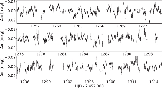
Figure 1. BRITE orbital-mean magnitudes of WR24 from the 36-Car-II field as a function of the Heliocentric Julian Date, after subtraction of the median, showing the stochastic photometric variability of this star.
Download figure:
Standard image High-resolution imageTable 1. BRITE Photometric Datasets of WR Stars Used in this Study
| Star | Spectral Type | Observing Interval | Satellite(s) | BRITE | α0 | νchar | γ | CW |
|---|---|---|---|---|---|---|---|---|
| (day) | Field Number | (mag) | (day−1) | (mag) | ||||
| WR6 (2015) | WN4-s | 157 | BTr | 12-CMaPup-I | 7.847e-04 | 0.537 | 1.406 | 1.515e-04 |
| WR22 (2017) | WN7h+O9V | 154 | BHr | 24-Car-I | 1.138e-03 | 0.543 | 2.348 | 1.913e-04 |
| WR22 (2018) | - | 150 | BHr-BTr | 36-Car-II | 9.517e-04 | 0.484 | 1.461 | 2.580e-04 |
| WR24 (2016) | WN6ha | 165 | BTr | 15-CruCar-I | 5.760e-04 | 0.433 | 1.233 | 2.036e-04 |
| WR24 (2017) | - | 154 | BTr | 24-Car-I | 2.315e-04 | 1.504 | 2.713 | 1.620e-04 |
| WR24 (2018) | - | 62 | BTr | 36-Car-II | 3.719e-04 | 0.983 | 2.447 | 2.869e-04 |
| WR40 (2018) | WN8h | 130 | BHr | 36-Car-II | 2.752e-03 | 0.583 | 1.987 | 3.271e-04 |
Download table as: ASCIITypeset image
The main advantage of BRITE photometry is the generally relatively long duration of the observations of each field, which ranges from 62 to 165 days for the data used in the present study. In particular, the longer among these runs allow for a much more accurate probing of the variability in the low-frequency range.
2.2. TESS Photometry
The TESS has a 90° × 24° FOV with its four main cameras and performs observations of stars in the 600–1000 nm range (Ricker et al. 2015). Its average observing interval on a specific field is ∼27 days, with either a 2 or 30 minute cadence for data collected during its prime mission. A 20 s cadence was added in the extended mission that started on 2020 July 5, along with a 10 minute cadence replacing the previous 30 minute cadence. Its accurate photometry makes this satellite ideal for observing short-term variability in the winds of WR stars in the ν ∈ [0.03, 350] days−1 domain. TESS data are publicly available on the Mikulski Archive for Space Telescopes (MAST) and can be accessed through various means. During the refereeing process of this paper, we became aware of another publication (Nazé et al. 2021) using a similar set of TESS observations to the one we are using in this study. They also report on the presence of red noise and discuss its characteristics.
We have retrieved all TESS data sets of single WR stars with a Gaia magnitude over 12 that were available on 2021 August 10. The details of the retrieved data sets are presented in Table 2, where we list the stars' names, their spectral types from the online WR catalog of P. Crowther (see references therein), the TESS sector in which the targets were located, the time intervals over which they were observed, the cadences used, and the fitted parameters of the semi-Lorentzian model described in Section 3.2. For each data set, we first checked for bright neighbors that could have contributed to the observed flux with the Gaia DR2 archive, and then cross-matched these with the Target Pixel Files (TPFs) also obtained through the Lightkurve package from the MAST, which shows how many pixels with length 21'' the source and neighbors occupy in the field. Stars with a bright, close-by (i.e., within a radius of less than 63'' from the target) visual neighbor were removed from our TESS sample, as were stars with bright visual neighbors further away that had a significant part of their flux smeared inside the 63'' radius around the target. We also did not include WR31b in our sample, as Groh et al. (2009) observed its spectral type varying from WN11h at minimum apparent magnitude of its S-Dor cycles to a type resembling an extreme A-type hypergiant at maximum visual magnitude, thus making it a different object than the cWR and WNh stars in our sample.
Table 2. TESS Photometric Datasets of WR Stars Used in this Study
| WR | Spectral | Observed TESS | Observing | Cadence | α0 | νchar | γ | CW |
|---|---|---|---|---|---|---|---|---|
| Type | Sector(s) | Interval | (minutes) | (mag) | (day−1) | (mag) | ||
| 1 | WN4b | 17–18 | 50.1 | 30 | 1.881e-03 | 0.362 | 1.501 | 2.884e-05 |
| 1 | WN4b | 24–25 | 52.4 | 30 | 6.614e-03 | 0.583 | 2.389 | 2.332e-05 |
| 3 | WN3ha | 18 | 23.7 | 2 | 5.452e-04 | 12.168 | 1.951 | 2.092e-05 |
| 3 | WN3ha | 18 | 24.3 | 30 | 4.201e-04 | 9.313 | 3.054 | 1.072e-04 |
| 4 | WC5+? | 18 | 23.5 | 2 | 1.861e-04 | 2.407 | 1.354 | 1.421e-05 |
| 4 | WC5+? | 18 | 24.3 | 30 | 2.902e-04 | 1.817 | 1.525 | 1.881e-06 |
| 5 | WC6 | 18 | 21.1 | 30 | 2.305e-04 | 1.490 | 1.149 | 6.796e-06 |
| 6 | WN4b | 6–7 | 47.8 | 2 | 2.341e-03 | 0.613 | 1.323 | 6.231e-06 |
| 6 | WN4b | 6–7 | 44.6 | 30 | 2.186e-03 | 0.525 | 1.439 | 8.907e-05 |
| 6 | WN4b | 33 | 25.8 | 2 | 1.781e-03 | 0.653 | 1.333 | 3.041e-06 |
| 6 | WN4b | 33 | 25.8 | 10 | 1.793e-03 | 0.646 | 1.321 | 9.691e-07 |
| 10 | WN5h | 7–8 | 50.4 | 30 | 8.581e-04 | 3.378 | 2.933 | 2.832e-05 |
| 10 | WN5h | 34 | 25.0 | 2 | 1.991e-03 | 2.657 | 2.198 | 2.672e-05 |
| 10 | WN5h | 34 | 25.3 | 10 | 1.491e-03 | 2.428 | 2.246 | 3.111e-05 |
| 13 | WC6 | 8–9 | 55.8 | 30 | 1.501e-04 | 1.455 | 1.624 | 3.428e-05 |
| 14 | WC7+? | 8–9 | 51.1 | 30 | 3.591e-04 | 0.652 | 0.882 | 1.851e-07 |
| 14 | WC7+? | 35–36 | 50.4 | 2 | 1.632e-04 | 2.361 | 1.399 | 4.904e-06 |
| 14 | WC7+? | 35–36 | 51.0 | 10 | 1.582e-04 | 2.509 | 1.573 | 8.391e-06 |
| 15 | WC6 | 8–9 | 50.8 | 30 | 6.891e-05 | 2.755 | 2.084 | 1.256e-05 |
| 15 | WC6 | 35–36 | 50.6 | 10 | 1.673e-04 | 0.769 | 1.097 | 7.901e-06 |
| 15 | WC6 | 35–36 | 60.4 | 2 | 1.403e-04 | 1.416 | 1.306 | 8.943e-06 |
| 16 | WN8h | 9–10 | 51.9 | 30 | 3.021e-03 | 0.681 | 1.796 | 5.132e-05 |
| 16 | WN8h | 36–37 | 51.0 | 2 | 7.523e-03 | 0.142 | 1.048 | 4.103e-07 |
| 16 | WN8h | 36–37 | 51.7 | 10 | 6.832e-03 | 0.152 | 1.049 | 3.883e-08 |
| 17 | WC5 | 9–10 | 51.7 | 30 | 1.402e-04 | 2.478 | 2.212 | 2.632e-05 |
| 17 | WC5 | 36 | 25.1 | 10 | 3.891e-04 | 0.677 | 0.907 | 1.712e-05 |
| 17 | WC5 | 36–37 | 51 | 2 | 1.674e-04 | 2.257 | 1.483 | 1.660e-05 |
| 22 | WN7ha+O9V | 10 | 26.0 | 2 | 1.686e-03 | 1.335 | 3.561 | 6.423e-06 |
| 22 | WN7ha+O9V | 10 | 26.0 | 30 | 1.976e-03 | 1.095 | 2.943 | 4.735e-05 |
| 22 | WN7ha+O9V | 36–37 | 25.3 | 2 | 1.662e-03 | 0.922 | 2.273 | 5.536e-06 |
| 22 | WN7ha+O9V | 36–37 | 25.3 | 10 | 1.922e-03 | 0.764 | 2.087 | 6.964e-06 |
| 23 | WC6 | 11 | 25.3 | 30 | 3.342e-04 | 0.803 | 1.034 | 9.623e-06 |
| 23 | WC6 | 36–37 | 51.0 | 2 | 1.143e-04 | 2.479 | 1.469 | 5.821e-06 |
| 23 | WC6 | 36–37 | 51.7 | 10 | 1.551e-04 | 1.133 | 1.095 | 6.001e-06 |
| 24 | WN6ha | 10 | 26.0 | 2 | 1.923e-03 | 1.096 | 1.872 | 8.542e-06 |
| 24 | WN6ha | 10–11 | 54.4 | 30 | 1.274e-03 | 1.096 | 1.982 | 1.504e-05 |
| 24 | WN6ha | 36–37 | 51.0 | 2 | 1.142e-03 | 1.606 | 2.613 | 3.702e-06 |
| 24 | WN6ha | 36–37 | 51.7 | 10 | 1.102e-03 | 1.679 | 2.821 | 7.234e-06 |
| 31a | WN11h | 10–11 | 54.4 | 30 | 3.339e-03 | 0.148 | 1.584 | 2.755e-05 |
| 33 | WC5 | 10 | 25.7 | 30 | 6.591 | 0.552 | 2.099 | 4.272e-05 |
| 33 | WC5 | 37 | 25.3 | 2 | 2.602e-04 | 1.044 | 1.516 | 5.081e-05 |
| 33 | WC5 | 37 | 25.2 | 10 | 2.272e-04 | 0.666 | 2.161 | 2.472e-05 |
| 40 | WN8h | 10 | 26.0 | 2 | 6.621e-03 | 0.861 | 1.931 | 1.553e-05 |
| 40 | WN8h | 10–11 | 54.4 | 30 | 6.982e-03 | 0.452 | 1.581 | 6.201e-05 |
| 40 | WN8h | 37-38 | 52.6 | 2 | 9.261e-03 | 0.385 | 1.451 | 5.152e-06 |
| 40 | WN8h | 37–38 | 53.3 | 10 | 1.021e-02 | 0.328 | 1.397 | 4.923e-06 |
| 46 | WN3b | 10 | 26.3 | 30 | 1.221e-02 | 0.545 | 3.209 | 7.942e-04 |
| 46 | WN3b | 33–34 | 53.3 | 2 | 2.551e-02 | 0.043 | 0.826 | 1.394e-08 |
| 46 | WN3b | 33–34 | 53.3 | 10 | 9.872e-03 | 0.163 | 0.867 | 9.553e-07 |
| 52 | WC4 | 11 | 27.1 | 30 | 1.992e-04 | 1.401 | 0.844 | 1.813e-07 |
| 52 | WC4 | 38 | 26.7 | 2 | 1.241e-04 | 4.104 | 1.601 | 9.264e-06 |
| 52 | WC4 | 38 | 26.7 | 10 | 1.912e-04 | 1.652 | 0.999 | 6.882e-06 |
| 53 | WC8d | 11 | 25.9 | 30 | 5.762e-04 | 1.009 | 1.252 | 2.244e-05 |
| 53 | WC8d | 38 | 26.7 | 2 | 3.221e-04 | 2.631 | 1.773 | 1.562e-05 |
| 53 | WC8d | 38 | 26.7 | 10 | 3.602e-04 | 2.058 | 1.421 | 1.560e-05 |
| 57 | WC8 | 11–12 | 54.9 | 30 | 1.862e-04 | 2.123 | 1.202 | 5.852e-06 |
| 57 | WC8 | 38 | 26.7 | 2 | 2.951e-04 | 2.121 | 1.408 | 1.281e-05 |
| 57 | WC8 | 38 | 26.7 | 10 | 3.281e-04 | 1.456 | 1.178 | 1.132e-05 |
| 60 | WC8 | 11 | 24.0 | 30 | 5.152e-04 | 0.631 | 2.406 | 3.420e-05 |
| 60 | WC8 | 38 | 26.7 | 2 | 2.211e-04 | 1.462 | 1.591 | 2.513e-05 |
| 60 | WC8 | 38 | 26.7 | 10 | 4.213e-04 | 0.289 | 1.391 | 1.801e-05 |
| 66 | WN8(h) | 12 | 27.9 | 30 | 1.923e-03 | 1.479 | 2.743 | 9.981e-05 |
| 66 | WN8(h) | 38 | 55.9 | 2 | 1.271e-03 | 1.743 | 2.195 | 1.541e-05 |
| 66 | WN8(h) | 38 | 55.9 | 10 | 1.721e-03 | 1.122 | 1.774 | 1.980e-05 |
| 67 | WN6o | 12 | 27.9 | 30 | 1.291e-02 | 0.198 | 0.987 | 9.912e-07 |
| 67 | WN6o | 38–39 | 55.9 | 2 | 1.061e-02 | 0.444 | 1.404 | 3.001e-05 |
| 67 | WN6o | 38–39 | 55.9 | 10 | 8.491e-03 | 0.507 | 1.472 | 7.291e-05 |
| 71 | WN6o | 12 | 27.9 | 30 | 1.942e-03 | 2.027 | 1.405 | 3.961e-05 |
| 71 | WN6o | 39 | 27.9 | 2 | 1.432e-03 | 3.649 | 1.905 | 1.641e-05 |
| 71 | WN6o | 39 | 27.9 | 10 | 1.971e-02 | 0.04 | 0.785 | 4.481e-08 |
| 75 | WN6b | 39 | 27.9 | 2 | 1.182e-03 | 0.545 | 1.698 | 1.941e-05 |
| 75 | WN6b | 39 | 21.8 | 10 | 6.241e-04 | 0.448 | 1.51 | 4.321e-05 |
| 78 | WN7h | 12 | 23.0 | 30 | 3.812e-03 | 0.707 | 1.805 | 3.313e-05 |
| 78 | WN7h | 39 | 27.9 | 2 | 2.572e-03 | 1.037 | 2.430 | 9.071e-06 |
| 78 | WN7h | 39 | 27.9 | 10 | 2.437e-03 | 1.230 | 3.120 | 2.032e-05 |
| 79b | WN9ha | 12 | 27.9 | 30 | 1.631e-03 | 1.579 | 3.761 | 4.401e-05 |
| 79b | WN9ha | 39 | 27.9 | 10 | 2.152e-03 | 1.242 | 2.653 | 2.132e-05 |
| 81 | WC9 | 12 | 22.9 | 30 | 4.391e-03 | 1.039 | 1.832 | 6.981e-05 |
| 87 | WN7h+abs | 12 | 23.0 | 30 | 6.263e-03 | 0.187 | 1.121 | 4.081e-06 |
| 87 | WN7h+abs | 39 | 27.9 | 2 | 2.071-03 | 1.309 | 2.962 | 1.951e-05 |
| 87 | WN7h+abs | 39 | 21.8 | 10 | 1.974e-03 | 0.957 | 2.302 | 6.85e-05 |
| 88 | WC9 | 12 | 23.0 | 30 | 6.242e-03 | 0.782 | 1.492 | 6.421e-05 |
| 88 | WC9 | 39 | 21.8 | 10 | 6.331e-03 | 1.150 | 2.171 | 6.971e-05 |
| 90 | WC7 | 12 | 27.9 | 30 | 4.001e-04 | 0.717 | 1.109 | 9.431e-06 |
| 90 | WC7 | 39 | 21.8 | 2 | 1.612e-04 | 2,691 | 1.354 | 4.471e-06 |
| 90 | WC7 | 39 | 21.8 | 10 | 5.621e-04 | 0.228 | 0.748 | 2.831e-08 |
| 92 | WC9 | 12 | 27.9 | 30 | 6.562e-03 | 0.616 | 1.328 | 2.681e-06 |
| 92 | WC9 | 39 | 21.8 | 10 | 4.204e-03 | 0.997 | 1.681 | 5.531e-05 |
| 94 | WN5o | 12 | 23.0 | 30 | 1.173e-03 | 0.350 | 0.961 | 2.241e-05 |
| 94 | WN5o | 39 | 27.6 | 2 | 2.271e-03 | 0.606 | 1.363 | 1.061e-05 |
| 95 | WC9d | 12 | 23.0 | 30 | 1.982e-03 | 1.300 | 1.518 | 6.781e-05 |
| 95 | WC9d | 39 | 21.8 | 10 | 1.682e-03 | 1.749 | 1.925 | 4.251e-05 |
| 100 | WN8o | 39 | 27.4 | 2 | 3.091e-03 | 0.987 | 1.746 | 6.112e-05 |
| 100 | WN8o | 39 | 21.8 | 30 | 3.023e-03 | 0.998 | 1.634 | 2.901e-05 |
| 103 | WC9d+? | 13 | 24.6 | 30 | 3.162e-03 | 1.336 | 1.842 | 3.431e-05 |
| 103 | WC9d+? | 39 | 27.5 | 2 | 3.591e-03 | 1.129 | 1.585 | 7.942e-05 |
| 103 | WC9d+? | 39 | 21.8 | 10 | 3.214e-03 | 1.298 | 1.628 | 1.831e-05 |
| 128 | WN4(h) | 14 | 26.8 | 30 | 1.061e-03 | 4.795 | 1.431 | 9.312e-06 |
| 130 | WN8h | 14 | 26.8 | 30 | 1.971e-03 | 0.967 | 2.143 | 4.901e-05 |
| 131 | WN7h+abs | 14 | 26.8 | 30 | 1.291e-03 | 1.199 | 3.523 | 8.132e-05 |
| 134 | WN6b | 14–15 | 54.0 | 30 | 1.542e-03 | 0.507 | 1.234 | 9.300e-06 |
| 135 | WC8 | 14–15 | 54.0 | 30 | 2.621e-04 | 1.512 | 1.298 | 8.991e-06 |
| 136 | WN6b(h) | 14–15 | 54.0 | 30 | 4.932e-04 | 0.798 | 2.352 | 1.841e-05 |
| 138a | WN8-9h | 14–15 | 54.0 | 30 | 1.890e-03 | 0.996 | 2.137 | 5.702e-05 |
| 142 | WO2 | 14–15 | 51.1 | 30 | 2.851e-04 | 0.425 | 1.395 | 3.161e-05 |
| 152 | WN3(h) | 16–17 | 51.0 | 30 | 5.720e-04 | 4.236 | 1.361 | 9.044e-07 |
| 154 | WC6 | 16 | 22.3 | 51.0 | 1.571e-04 | 1.496 | 1.478 | 1.752e-05 |
| 158 | WN7h | 17–18 | 50.3 | 30 | 1.610e-03 | 1.438 | 2.849 | 3.541e-05 |
| 158 | WN7h | 24 | 26.4 | 30 | 4.231e-03 | 0.627 | 1.575 | 6.899e-07 |
| 159 | WN7h | 17–18 | 50.3 | 30 | 3.021e-03 | 0.255 | 1.782 | 3.702e-05 |
| 159 | WN7h | 24 | 26.4 | 30 | 3.592e-03 | 0.313 | 1.695 | 3.911e-05 |
The 2 minute TESS lightcurves, which have been detrended by the TESS data pipeline following Jenkins et al. (2016), were obtained from the MAST using the Lightkurve package for Python (Lightkurve Collaboration et al. 2018), while the 10 and 30 minute TESS lightcurves were extracted from the TPFs. Aperture photometry with a custom mask for the source was performed on each data set, with a flux threshold usually in the range of 7–10 median absolute deviations (MADs) above the median flux, but sometimes lower for fainter sources or higher in the case where another bright star is present in the field. A background mask was defined by pixels with a median flux value of 10−4 MADs or less, and the background signal was subsequently subtracted from the source. A principal component analysis was then performed to remove the remaining instrumental noise and systematics from each data set, using the Lightkurve Regression Corrector method. An example of the resulting photometry (with the median value subtracted) is shown as a function of the Barycentric TESS Julian Date (BTJD) in Figure 2, where we present the 30 minute cadence TESS lightcurve of the WN8h star WR40.

Figure 2. 30 minute cadence TESS lightcurve of WR40 after subtraction of the median magnitude. BTJD stands for "Barycentric Tess Julian Date".
Download figure:
Standard image High-resolution image2.3. MOST Photometry
The MOST satellite (Matthews 2003, 2004; Walker et al. 2003) housed a 15 cm optical telescope feeding a CCD photometer through a single custom broadband (400–700 nm) filter. MOST followed a polar Sun-synchronous orbit at 820 km altitude, enabling it to monitor stars in its equatorial continuous viewing zone for up to 8 weeks without interruption with a cadence of ∼100 minutes.
Our sample includes six single WR stars observed with MOST, which are listed in Table 3 along with their spectral types, observing interval, and fitted parameters of the semi-Lorentzian model described in Section 3.2. However, only WR92, 103, 115, and 120 still had data files available with parameters related to the satellite's onboard instruments, allowing us to carry out detrending procedures following Pigulski et al. (2016). The other stars' data had already been reduced by previous users, though not published, and thus were used without further modification. As an example, we present the MOST lightcurve of the WN7o star WR120 in Figure 3.
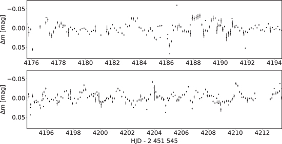
Figure 3. MOST lightcurve of WR120 after removal of the overall median flux.
Download figure:
Standard image High-resolution imageTable 3. MOST Photometric Datasets of WR Stars Used in this Study
| Star | Spectral Type | Observing Interval | α0 | νchar | γ | CW |
|---|---|---|---|---|---|---|
| [day] | (mag) | (day−1) | (mag) | |||
| WR71 | WN6o | 26.8 | 4.810e-03 | 0.291 | 0.855 | 1.190e-04 |
| WR92 | WC9 | 26.3 | 5.459e-04 | 2.791 | 0.911 | 2.239e-05 |
| WR103 | WN9d+? | 37.2 | 1.879e-03 | 1.156 | 2.488 | 1.388e-04 |
| WR115 | WN6o | 37.8 | 1.629e-04 | 0.224 | 0.873 | 3.122e-04 |
| WR119 | WC9d | 47.7 | 3.055e-03 | 0.259 | 2.064 | 7.071e-04 |
| WR120 | WN7o | 37.8 | 9.584e-04 | 1.170 | 4.764 | 8.506e-04 |
Download table as: ASCIITypeset image
3. Data Analysis
3.1. Frequency Analysis
All the lightcurves analyzed in this work are made available as online material. In order to characterize them, we first carried out period searches to identify the dominant frequencies present in the photometry of each star. For this, we used the discrete Fourier transform method implemented in the PERIOD04 software (Lenz & Breger 2005) to obtain periodograms for each data set of all stars in our sample. These are also available as online material.
As we are interested in the stochastic variability of these WR stars, we first had to remove any a priori known periodicities from our observations before carrying out our analysis, a process known as prewhitening. This was done by evaluating the amplitude signal-to-noise ratio (S/N) of each peak corresponding to a known periodicity in the stars' periodograms. The S/N is calculated as the ratio of the peak amplitude over the average amplitude of residuals inside a symmetric 1 day−1 window around the frequency of the peak, following the methodology given in the Methods section of Bowman et al. (2019a). If the S/N value of a peak is above four, the peak is deemed significant, as suggested by Breger et al. (1993), and the corresponding signal is removed by fitting the sinusoidal model,

on the lightcurve of time, t, normalized to a zero-point, t0, with a phase-shift, ϕ, while using the peak's frequency ν and amplitude A.
The BRITE sample contains two stars, WR6 and WR22, with known periodic signals which are expected to exhibit distinct individual peaks in their periodograms. WR6 presents variations in photometry, polarimetry and spectroscopy with a period of 3.76 days that could be explained by the presence of CIRs in its wind (e.g., Morel et al. 1997), although, e.g., Schmutz & Koenigsberger (2019) prefer a binary scenario. In view of the epoch dependency of the variability and the length of the lightcurve, a tailored iterative prewhitening procedure was conducted for WR6 by first carrying out a time-dependent frequency (TF) analysis (also known as Gabor transform) to localise the time intervals over which the various harmonics of the 3.76 day signal are present. We then removed the harmonics with S/N over four by fitting the sinusoidal function previously described in the corresponding time interval and subtracting the fit from the portion of the lightcurve containing the signals. The amplitude and frequencies of the removed harmonics are shown in Table 4. Also, WR22 is a well-known eclipsing binary with a period of 80 days, whose eclipse has recently been modeled by Lenoir-Craig et al. (2021). We used their best-fit Model 1 using the O9V spectral class for the companion to remove two eclipses from the 2017 data and one from the 2018 observation run.
Table 4. Various Signals Removed from the Datasets Used in this Study
| Star | Sector/Field | Cadence/Satellite | (ν [day−1], Amplitude [mag]) |
|---|---|---|---|
| WR1 | 17–18 | 30 | (5.670e-02, 5.355e-03) |
| WR3 | 18 | 30 | (0.193, 1.968e-03) |
| WR6 | 12-CMaPup-I | BTr | (0.2729, 0.0124), (0.5314, 0.0100), (0.7870, 0.0057), |
| (1.0649, 0.0058) | |||
| WR6 | 6–7 | 2 | (0.267, 1.071e-02), (0.529, 2.674e-02), (0.794, 1.077e-02) |
| WR6 | 6–7 | 30 | (0.2522, 0.0110), (0.5294, 2.651e-02), (0.7844, 0.0089) |
| (1.3224, 2.448e-03) | |||
| WR6 | 33 | 2 | (0.267, 1.213e-02), (0.532, 7.245e-03), (0.799, 5.231e-05) |
| WR6 | 33 | 10 | (0.267, 1.211e-02), (0.531, 7.274e-03), (0.800, 5.212e-05) |
| WR10 | 34 | 2 | (0.496, 5.047e-03) |
| WR10 | 34 | 10 | (0.498, 3.602e-03), (7.988, 5.026e-04) |
| WR13 | 8–9 | 30 | (0.318, 6.653e-04), (0.587, 6.659e-04) |
| WR14 | 18 | 2 | (208.646, 4.457e-05), (329.786, 5.331e-05) |
| WR15 | 35–36 | 2 | (313.151, 3.569e-05) |
| WR16 | 36–37 | 2 | (3.824e-02, 1.137e-02) |
| WR16 | 36–37 | 10 | (3.771e-02, 1.080e-02) |
| WR17 | 9–10 | 30 | (0.496, 4.790e-04) |
| WR17 | 36–37 | 2 | (58.602, 6.715e-05) |
| WR17 | 36 | 10 | (9.774, 1.550e-05), (49.036, 9.796e-05) |
| WR33 | 10 | 30 | (2.879, 1.568e-04) |
| WR33 | 37 | 2 | (204.054, 1.736e-04) |
| WR33 | 37 | 10 | (16.491, 1.692e-04) |
| WR40 | 10 | 2 | (0.212, 1.710e-02) |
| WR46 | 10 | 30 | (3.064, 6.873e-03), (6.557, 1.362e-02) |
| WR46 | 37-38 | 2 | (2.956, 6.338e-03), (3.253, 8.925e-03), (3.271, 5.702e-03), |
| (3.282, 2.012e-02), (3.303, 1.170e-02), (3.329, 8.627e-03), | |||
| (3.582, 4.441e-03), (6.249, 7.708e-03), (6.325, 5.956e-03), | |||
| (6.583, 2.625e-02), (6.879, 6.953e-03), (6.921, 9.380e-03), | |||
| (7.698, 2.659e-03), (9.871, 2.992e-03), (10.215, 2.686e-03), | |||
| (12.951, 2.369e-03) | |||
| WR46 | 37–38 | 10 | (2.9564, 4.882e-03), (3.2559, 7.848e-03), (3.2813, 1.662e-02), |
| (3.307, 6.696e-03), (3.330, 9.927e-03), (6.248, 6.459e-03), | |||
| (6.326, 4.927e-03), (6.583, 2.164e-02), (6.880, 5.965e-03), | |||
| (6.920, 7.989e-03), (7.698, 2.223e-03), (9.872, 2.546e-03), | |||
| (10.216, 1.364e-03), (12.950, 2.017e-03) | |||
| WR52 | 38 | 2 | (201.449, 3.389e-05), (298.668, 3.656e-05), (334.010, 3.524e-05) |
| WR53 | 38 | 2 | (294.865, 4.961e-05), (312.260, 5.614e-05) |
| WR53 | 38 | 10 | (0.171, 1.687e-03), (5.698, 3.832e-04), (7.054, 3.785e-04) |
| WR57 | 38 | 2 | (20.887, 7.277e-05) |
| WR66 | 12 | 30 | (0.816, 6.291e-03), (3.791, 1.015e-03), (5.426, 3.246e-03), |
| (6.074, 3.118e-03), (6.826, 1.814e-03), (6.928, 4.902e-03) | |||
| (7.435, 9.415e-04), (7.741, 6.784e-04), (12.999, 6.577e-04) | |||
| WR66 | 38–39 | 2 | (1.647, 3.352e-03), (4.692, 7.683e-04), (5.427, 3.207e-03), |
| (6.075, 3.779e-03), (6.257, 7.649e-04), (6.827, 1.745e-03), | |||
| (6.927, 5.440e-03), (7.434, 1.115e-03), (7.537, 4.473e-04), | |||
| (8.851, 8.110e-04), (10.853, 4.003e-04), (13.002, 8.441e-04), | |||
| (13.186, 2.002e-04), (13.853, 5.169e-04), (15.779, 1.682e-04), | |||
| (19.927, 1.538e-04) | |||
| WR66 | 38-39 | 10 | (1.647, 3.192e-03), (3.291, 1.103e-03), (3.782, 7.162e-04), |
| (4.694, 7.216e-04), (5.427, 3.002e-03), (6.075, 3.560e-03), | |||
| (6.257, 7.474e-04), (6.827, 1.662e-03), (6.927, 5.122e-03), | |||
| (7.435, 1.073e-03), (7.538, 4.163e-04), (8.852, 7.537e-04), | |||
| (10.852, 3.927e-04), (13.002, 7.924e-04), (13.853, 4.745e-04) | |||
| WR67 | 39 | 2 | (6.548, 2.122e-03) |
| WR67 | 39 | 10 | (6.548, 2.005e-03) |
| WR71 | 39 | 2 | (0.392, 3.563e-03), (0.533, 2.749e-03) |
| WR71 | 39 | 10 | (0.385, 8.130e-03) |
| WR75 | 39 | 2 | (188.898, 7.101e-05) |
| WR75 | 39 | 10 | (0.124, 3.507), (45.943, 1.526e-04) |
| WR87 | 12 | 30 | (8.922e-02, 7.404e-03) |
| WR90 | 39 | 10 | (0.101, 7.755e-04) |
| WR92 | 39 | 10 | (0.124, 1.044e-02), (6.721, 8.956e-04) |
| WR94 | 39 | 10 | (6.872e-02, 5.401e-03), (0.108, 8.096e-03), (0.142, 2.222e-03), |
| (0.211, 3.857e-03) | |||
| WR95 | 12 | 30 | (5.953, 9.580e-04) |
| WR100 | 39 | 2 | (6.662, 1.170e-03), (8.680, 1.642e-03), (13.335, 2.138e-04), |
| (15.349, 4.230e-04), (17.350, 2.780e-04) | |||
| WR134 | 14–15 | 30 | (0.437, 6.000e-03), (0.881, 3.512e-03) |
| WR135 | 14–15 | 30 | (2.712, 4.419e-04), (5.445, 1.971e-04), (5.470, 2.874e-04), |
| (8.197, 1.436e-04) | |||
| WR142 | 14–15 | 30 | (0.296, 1.981e-03), (0.592, 1.412e-03), (11.679, 4.557e-04) |
| WR158 | 17–18 | 30 | (9.542e-02, 5.823e-03), (1.004, 4.653e-03) |
| WR159 | 17–18 | 30 | (4.371e-02, 9.668e-03) |
In the TESS sample, eight stars are known to show periodic signals that could be detected within TESS's ∼27 days sectors: WR1, 6, 22, 46, 66, 100, 103, and 134. WR1 and WR134 are both highly likely to harbor CIRs in their winds, with the former exhibiting variations in both spectroscopy and photometry with a period of 16.9 days (Chené & St-Louis 2010), while the spectroscopic variability of the latter shows a clear periodicity of 2.3 days (McCandliss et al. 1994; Morel et al. 1999). The causes of the observed short-term periodic variabilities of WR46 (P ∼ 8 hr) and WR66 (P ∼ 4 hr) are still uncertain, with plausible scenarios ranging from nonradial pulsations to close binaries with compact objects (Antokhin et al. 1995; Hénault-Brunet et al. 2011; Gosset et al. 2011; Skinner et al. 2021). Spectroscopic observations of WR100 were conducted by Chené & St-Louis (2011), and CIR-type large-scale line-profile variability has been observed in its winds, albeit without the determination of a clear period. Chené & St-Louis (2011) also investigated spectroscopic observations of WR103, and small-scale line-profile variability was detected, again with no clear period detected. Except for WR103, significant peaks were detected near the expected frequencies (and sometimes harmonics) for all of these stars, with the frequencies and amplitudes of the removed signals shown in Table 4. Also, we completely removed the eclipse data from the TESS sector 36 observations of WR22, as the shape of the TESS-observed eclipse is sufficiently different from the ones observed by BRITE to require it to be numerically modeled separately to ensure a correct detrending, which goes beyond the scope of the present study.
Three stars in the MOST sample are also known to exhibit periodic signals: WR103, 115, and 120, with the latter two exhibiting large-scale CIR-type variability in spectroscopic observations (Chené & St-Louis 2011), with no clear detected periodicity. No significant peak were detected in the periodograms of any of the corresponding data sets.
Once the known significant periodicities were removed, the same procedure was iteratively repeated for all other peaks with S/N bigger than four in all of our sample stars' periodograms, again following the details given in the Methods section of Bowman et al. (2019a). Many more significant signals were removed from multiple TESS lightcurves, with their frequencies and amplitudes shown in Table 4.
A thorough analysis of all the WR periodograms in our sample revealed no other outstanding peak than those described in Table 4. The periodograms all show a forest of a large number of peaks with an increasing amplitude toward lower frequencies, starting from ∼0.5 day−1 down to ∼0.1 day−1, sometimes followed by a decrease in amplitude below 0.1 day−1, similarly to what had been observed by Ramiaramanantsoa et al. (2019) for the WN8 star WR40. This decrease in amplitude is presumably intrinsic to the stars, being unrelated to any details of the detrending process. An example of an amplitude spectrum we obtained for the WN6ha star WR24 is shown in Figure 4. All amplitude spectra are available as online material.

Figure 4. Amplitude spectrum of WR24 as observed by BHr in 2017 (black solid line). The solid green line corresponds to the fit of the semi-Lorentzian distribution, with the red- and white-noise components, respectively, shown as red and blue dashed lines.
Download figure:
Standard image High-resolution image3.2. Fit of the Stochastic Variability
In order to characterize the stochastic, low-frequency variability for our sample of WR stars, we fitted a combination of red and white noise to all our amplitude spectra as described, for example, in Bowman et al. (2019a) or Bowman et al. (2019b), by applying a Markov Chain Monte Carlo algorithm using the Python code Emcee (Foreman-Mackey et al. 2013) to fit the amplitude spectrum of each lightcurve with a semi-Lorentzian distribution:
where α0 represents the amplitude of the frequency-dependent component in the limit of zero frequency; νchar is the characteristic frequency of the stochastic variability present in the lightcurve, which is the inverse of the characteristic timescale following νchar = (2π τ)−1; and γ is the logarithmic amplitude gradient. The first term on the right-hand side of this equation corresponds to the frequency-dependent red noise, while the second term, CW , is the frequency-independent white noise. It is important to note that the values of fitted α0 are significantly higher than the error bars of the photometric observations, and therefore are actually genuine intrinsic signals from the star and not noise in the traditional sense (see Bowman et al. 2019a). The white-noise components, however, are of much smaller amplitude, lower than or of the same level as the error bars, and are more likely to correspond mainly to instrumental or photon noise. Similarly to Bowman et al. (2019a), we then tested the goodness of the fit against a white-noise-only model using statistical F-tests. In all cases, we found the red-noise component to be significant. An example of such a fit to an amplitude spectrum is shown in Figure 4 for WR24 superposed on the observations plotted in black. The red- and white-noise components are plotted as red and blue dashed curves, respectively, while the resulting fit is shown as a solid green curve. All other fits can be found superposed on the amplitude spectra in the online material, and all the fitted parameters are listed in Tables 1, 2 and 3. We note that the values of our fitted parameters are in agreement with the range of red-noise parameters for WR stars shown in Figure 4 of the recent work done by Nazé et al. (2021) on the presence of red noise in the photometric data of evolved massive stars.
In order to check for trends between the values of the fitted model parameters and multiple stellar characteristics, we first had to ensure the comparability of the data. The data we are using in this study have been acquired by three different telescopes observing with various cadences in neighboring and/or overlapping wavelength ranges in the visible and very-close (700–1000 nm) infrared parts of the spectrum over different observation periods. Fortunately, it is well established that the source of visible continuum light for WR stars is wavelength-independent electron scattering in the winds, and therefore we do not expect that the different observation bands will significantly impact the observed fluxes, periodograms and fitted model parameters. Also, the duration of the observational data determines the lowest detectable frequency in the amplitude spectra, which for data covering multiple weeks will always be below the frequency range over which the red noise is observed (∼0.1–0.5 day−1). Therefore, this should also not significantly affect the fitted parameters.
However, the different sampling rates of the telescopes are expected to influence the values of the fitted model parameters, and a vital step here is to quantify by how much. To do this, we used all TESS lightcurves with a 2 minute cadence in our sample and created as many lightcurves with a uniform sampling of 10, 30, and 100 minutes as possible from them. We had to exclude the 2 minute lightcurves from WR3, 4, 33, and 60 from the 100 minute lightcurve creation process, as some of the lightcurves created from them showed no red noise in their periodograms. We were thus able to create 170, 510, and 1500 lightcurves with, respectively, 10, 30, and 100 minute cadences from our 34 original 2 minute lightcurves. We then fitted the red and white noise semi-Lorentizan model from Equation (2) on their periodograms, extracted the optimal model parameters, and normalized α0, νchar, and γ by the original best-fit parameter value of the 2 minute lightcurve. We show in Figure 5 the averages and standard deviations of all parameters for the different cadences.
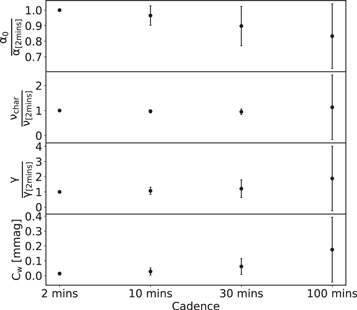
Figure 5. Fitted parameters of the semi-Lorentzian model applied on TESS lightcurves with cadences corresponding or close to those of the various data in our overall sample of WR stars. The lightcurves with 10, 30, and 100 minute cadences were created from the 2 minute ones. The average values of α0, νchar, and γ have been normalized by the parameter value of the original 2 minute lightcurve and are shown by a black dot, while the error bars correspond to a standard deviation from the average.
Download figure:
Standard image High-resolution imageWe observe from Figure 5 that the fitted value of α0 seems to follow a negative trend with increasing standard deviation as the cadence goes down. The 10 minute lightcurves have  , the 30 minute lightcurves have
  and the 100 minute lightcurves have
  . We remark that the means of the 10, 30, and 100 minute cadences always stay within one standard deviation of the 2 minute value. From this, we can estimate an intrinsic uncertainty on the value of α0 for cadences lower than 2 minutes, which is ±6% for 10 minute cadences, ±13% for 30 minute cadences, and ±27% for 100 minute cadences. However, as shown in Figures 6 and 7, these uncertainties on α0 for lightcurves with 10, 30, and 100 minute cadences are negligible when compared to the uncertainty brought forth by the varying values of fitted parameters over different epochs of observation, as the structures in the winds of the WR stars are changing over time, affecting the level of electron scattering.
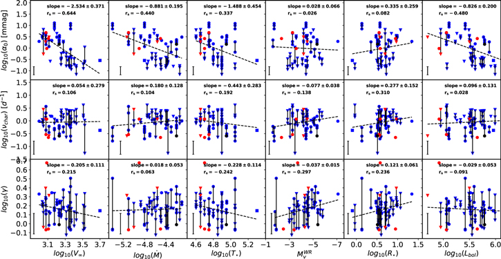
Figure 6. For the sample including WR stars without signs of H in their spectrum, fitted parameters of the red-noise component, α0, νchar, and γ as a function of various wind and stellar parameters, v∞ in km s−1,  in M⊙ yr–1, T in kK, R⋆ in R⊙, and Lbol in units of L⊙. Blue points are for TESS data, black for BRITE and red for MOST. The different data sets of individual stars observed by the same telescope are linked by black lines. Inverted triangles are for WC stars, and filled circles are for WN stars. The slope of the fitted straight line together with its error is given in the top-right corner of each panel along with the Spearman correlation coefficient, rs
. The size of the average standard deviation representing the intrinsic change of parameters characterizing the red-noise component for stars observed multiple times over different epochs are shown in the bottom-left corner of each panel.
in M⊙ yr–1, T in kK, R⋆ in R⊙, and Lbol in units of L⊙. Blue points are for TESS data, black for BRITE and red for MOST. The different data sets of individual stars observed by the same telescope are linked by black lines. Inverted triangles are for WC stars, and filled circles are for WN stars. The slope of the fitted straight line together with its error is given in the top-right corner of each panel along with the Spearman correlation coefficient, rs
. The size of the average standard deviation representing the intrinsic change of parameters characterizing the red-noise component for stars observed multiple times over different epochs are shown in the bottom-left corner of each panel.
Download figure:
Standard image High-resolution imageνchar appears to be the parameter least influenced by a changing cadence in Figure 5, with a relatively constant mean and increasing uncertainty as cadence goes down. It is important to note that the error bars of the average 100 minutes value of νchar, γ, and CW are overestimated due to their non-normal distributions. The γ and CW parameters exhibit a similar behavior to one another, both showing an increase in their values and spread as the cadence gets lower. This was expected for CW , since white noise is known to be dependent on the satellite cadence of observations and on the photometric precision (Bowman et al. 2020). As with α0, the values of the intrinsic errors on the parameters due to the cadence for the 10, 30, and 100 minute lightcurves are negligible when compared with the typical variations of these parameters between different epochs, as shown in Figures 6 and 7.
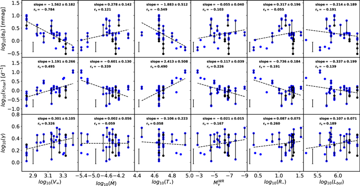
Figure 7. For WN stars with signs of H in their spectrum, fitted parameters of the red-noise component, α0, νchar, and γ as a function of various wind and stellar parameters, v∞ in kms−1,  in M⊙ yr–1, T in kK, R⋆ in R⊙, and Lbol in units of L⊙. Blue points are for TESS data, black for BRITE and red for MOST. The different data sets of individual stars observed by the same telescope are linked by black lines. Inverted triangles are for WC stars and filled circles are for WN stars. The slope of the fitted straight line together with its error is given in the top-right corner of each panel along with the Spearman's rank correlation coefficient, Rs
. The size of the average standard deviation representing the intrinsic change of parameters characterizing the red-noise component for stars observed multiple times over different epochs are shown in the bottom-left corner of each panel.
in M⊙ yr–1, T in kK, R⋆ in R⊙, and Lbol in units of L⊙. Blue points are for TESS data, black for BRITE and red for MOST. The different data sets of individual stars observed by the same telescope are linked by black lines. Inverted triangles are for WC stars and filled circles are for WN stars. The slope of the fitted straight line together with its error is given in the top-right corner of each panel along with the Spearman's rank correlation coefficient, Rs
. The size of the average standard deviation representing the intrinsic change of parameters characterizing the red-noise component for stars observed multiple times over different epochs are shown in the bottom-left corner of each panel.
Download figure:
Standard image High-resolution image3.3. Search for Correlations
We then looked for correlations between the parameters describing the red-noise component of the photometric changes observed in our stars with various stellar and wind parameters. In order to do so, we first separated our sample into two separate groups, one including stars that showed signs of the presence of hydrogen in their spectra, and the other including stars that did not. In Figures 6 and 7, we present log-log plots of α0, νchar, and γ, all provided in Tables 1–3, as a function of the wind terminal velocity, mass-loss rate, stellar temperature, absolute magnitude in the Smith v band,  , stellar radius, and bolometric luminosity. The stellar radius, R*, in this context refers to the location where the Rosseland continuum optical depth is equal to τRoss,c
= 20, and the stellar temperature, T*, is the fictitious quantity calculated using the Stefan–Boltzmann relation at that position, as was done in Hamann et al. (2019) and Sander et al. (2019). TESS data are in blue, BRITE data in black and MOST data are in red, with WC stars indicated by circles, WN stars by inverted triangles and the WO2 star WR142 by a square. The wind and stellar parameters were taken from Hamann et al. (2019) for WN stars and Sander et al. (2019) for WC and WO stars, and the absolute magnitudes were taken from Rate & Crowther (2020). For WR79b, the stellar parameters were taken from Bohannan & Crowther (1999), and for WR138a from Gvaramadze et al. (2009), as these stars did not figure in the previously mentioned references. For the three stars in our sample for which no individual values were available, namely WR8, 87, and 159, we used the average value for stars of the same spectral type from Hamann et al. (2019). Note that recently there have been great strides made in the understanding of how the optically thick winds of WR stars are launched and driven. Grassitelli et al. (2018) presented one-dimensional hydrodynamic stellar structure models for He stars that demonstrate that outflows can be driven to supersonic velocities by the opacity associated to the recombination of Fe atoms, the so-called Fe-peak opacities (at T ∼ 200kK) and/or the He ii opacity bump (at T ∼ 50 kK). They find that above a given
, stellar radius, and bolometric luminosity. The stellar radius, R*, in this context refers to the location where the Rosseland continuum optical depth is equal to τRoss,c
= 20, and the stellar temperature, T*, is the fictitious quantity calculated using the Stefan–Boltzmann relation at that position, as was done in Hamann et al. (2019) and Sander et al. (2019). TESS data are in blue, BRITE data in black and MOST data are in red, with WC stars indicated by circles, WN stars by inverted triangles and the WO2 star WR142 by a square. The wind and stellar parameters were taken from Hamann et al. (2019) for WN stars and Sander et al. (2019) for WC and WO stars, and the absolute magnitudes were taken from Rate & Crowther (2020). For WR79b, the stellar parameters were taken from Bohannan & Crowther (1999), and for WR138a from Gvaramadze et al. (2009), as these stars did not figure in the previously mentioned references. For the three stars in our sample for which no individual values were available, namely WR8, 87, and 159, we used the average value for stars of the same spectral type from Hamann et al. (2019). Note that recently there have been great strides made in the understanding of how the optically thick winds of WR stars are launched and driven. Grassitelli et al. (2018) presented one-dimensional hydrodynamic stellar structure models for He stars that demonstrate that outflows can be driven to supersonic velocities by the opacity associated to the recombination of Fe atoms, the so-called Fe-peak opacities (at T ∼ 200kK) and/or the He ii opacity bump (at T ∼ 50 kK). They find that above a given  , the winds can be driven entirely by Fe. For winds that cannot, the additional He ii opacities result in an extended low-density envelope accompanied by a density inversion. The stars that launch these Fe-driven winds all have a very compact core, close to 1 R⊙. Until very recently, this result was in contrast with results of stellar atmosphere codes that estimated radii higher by a factor of 2–3. However, Sander et al. (2020) have now produced improved atmosphere models for classical WR stars in which the hydrodynamical equation of motion is solved throughout the atmosphere. They find, in accord with Grassitelli et al. (2018), that the winds are driven by the peak in the Fe opacities. Furthermore, they also show that the complex ionization structure of the wind that helps to drive the wind in the outer layers results in complex velocity laws that cannot be well described by a simple beta law. Similar conclusions were reached by Poniatowski et al. (2021) using a combination of static OPAL opacities usually used in static stellar structure models with a simple parameterization equation to take into account the additional line opacity from a supersonic flow. These velocity laws are found to include bumps, plateaus, and even deceleration regions. This is an important result because the stellar parameters, and in particular the stellar temperature, that have been derived in the papers we have used are based on using a beta law to relate quantities in the observable part of the wind to those at the stellar surface. At the present time, no updated values of these stellar parameters are available and it is unclear what the effect of assuming a beta law is on the published parameters
11
we have used to search for correlations. Obviously, once new values become available, the study will have to be redone.
, the winds can be driven entirely by Fe. For winds that cannot, the additional He ii opacities result in an extended low-density envelope accompanied by a density inversion. The stars that launch these Fe-driven winds all have a very compact core, close to 1 R⊙. Until very recently, this result was in contrast with results of stellar atmosphere codes that estimated radii higher by a factor of 2–3. However, Sander et al. (2020) have now produced improved atmosphere models for classical WR stars in which the hydrodynamical equation of motion is solved throughout the atmosphere. They find, in accord with Grassitelli et al. (2018), that the winds are driven by the peak in the Fe opacities. Furthermore, they also show that the complex ionization structure of the wind that helps to drive the wind in the outer layers results in complex velocity laws that cannot be well described by a simple beta law. Similar conclusions were reached by Poniatowski et al. (2021) using a combination of static OPAL opacities usually used in static stellar structure models with a simple parameterization equation to take into account the additional line opacity from a supersonic flow. These velocity laws are found to include bumps, plateaus, and even deceleration regions. This is an important result because the stellar parameters, and in particular the stellar temperature, that have been derived in the papers we have used are based on using a beta law to relate quantities in the observable part of the wind to those at the stellar surface. At the present time, no updated values of these stellar parameters are available and it is unclear what the effect of assuming a beta law is on the published parameters
11
we have used to search for correlations. Obviously, once new values become available, the study will have to be redone.
We fitted a straight line to all these data sets using a least-squares algorithm and overplotted the result as a dashed black line. The value of the slope and its corresponding error is given in the top-right corner of each panel along with the Spearman's rank Rs coefficient. If more than one data set existed for a given star, we linked the fitted values of the parameters describing the red-noise component with a vertical line to show the range covered by the values we obtain for the various observations.
There are seven graphs in Figures 6 and 7 that have slopes above the 3σ level and a two-sided Spearman's rank coefficient that is significant at p < 0.001 for the number of points in our samples. However, only the negative trend between  (we refer to log10 as
  throughout the text) and logv∞ also has a significant p-value at the p < 0.05 level associated with an F-test between the χ2 of the fitted linear trend and the χ2 of a best-fit flat model for both cWR and WNh stars. Thus, although we can determine the presence of correlations for the six other graphs, we cannot ascertain their statistical significance with our current sample.
Correlations satisfying the Spearman's rank p < 0.001 criterion for the correlation coefficient, rs
, are observed between  and both
  and
and  in Figure 6, indicating that hotter (since v∞ and T* are related), more-luminous cWRs with denser winds appear to exhibit lower levels of stochastic variability than their cooler counterparts. We note here that the Spearman's rank of
  versus
  is just slightly under the threshold. We also note that the negative correlation between
  and
and  is contrary to the results of Bowman et al. (2020) for OB stars, who found that higher-luminosity stars tend to be characterized by larger values of α0.
For WNh stars, correlations are observed between  and
and  , and also between
  and both
  and
and  . An important remark to make here is that these last two trends drop below of the Spearman's rank coefficient if the TESS data from WR3 is removed from the sample, as its two data sets observed over different periods both have a fitted γ > 9, by far the highest values of our sample, with the next highest value being γ ∼ 4.7, and the overall (cWR + WNh) mean and standard deviation being 1.7 ± 0.8. Since a close inspection of the data and procedure has not revealed anything anomalous, and since the periodograms of both independently observed epochs have been fitted with such a high γ, we consider it real and not an erroneous observation. Note also that T* and v∞ are known to be correlated: hotter stars tend to have faster winds, although this has not been formally quantified (e.g., Hamann et al. 2019). As previously mentioned, we can also observe in Figures 6 and 7 that for stars that have been observed over different epochs, the fitted coefficients can be significantly different from one observation to the next, even when they are observed with the same satellite. We consider that this is real scatter and most likely represents a change in the conditions in the wind that must be taken into account. We therefore estimated a standard deviation characterizing these changes as follows:

where ni
is the number of different observations of the ith star,  corresponds to the standard deviation of the chosen parameter calculated over the ni
observations of that same star, while N corresponds to the total number of observations of stars that have been observed multiple times. The resulting values are plotted in the bottom-left corner of each panel in Figures 6 and 7. Using these values as error bars for our F-tests, we find one significant correlation at p < 0.05 between α0 and v∞ for all WR stars, with corresponding p-values of 0.02 for cWR and 7 × 10⁻⁴ for WNh. We believe that this trend should be investigated further, as should be the other observed correlations once more data sets are acquired and the range of intrinsic change of the various parameters is better established. We also note that a similar trend between spectroscopic variability and T* was found in spectroscopic data sets of WR stars by Chené et al. (2020).
corresponds to the standard deviation of the chosen parameter calculated over the ni
observations of that same star, while N corresponds to the total number of observations of stars that have been observed multiple times. The resulting values are plotted in the bottom-left corner of each panel in Figures 6 and 7. Using these values as error bars for our F-tests, we find one significant correlation at p < 0.05 between α0 and v∞ for all WR stars, with corresponding p-values of 0.02 for cWR and 7 × 10⁻⁴ for WNh. We believe that this trend should be investigated further, as should be the other observed correlations once more data sets are acquired and the range of intrinsic change of the various parameters is better established. We also note that a similar trend between spectroscopic variability and T* was found in spectroscopic data sets of WR stars by Chené et al. (2020).
3.4. Wavelet Analysis
In order to obtain a different perspective on the timescales of the variability present in our photometric observations, we carried out wavelet analyses on all data sets for the stars in our sample following the method of Torrence & Compo (1998). An example is shown in Figure 8 for the TESS data of WN6ha star WR24. The top panel shows a reconstruction of the lightcurve of this star using 60 minute bins, and the bottom panel shows the wavelet power-spectrum of this data set. We find that the stronger signals have periods in the 1–5 days range. This is consistent with the results of our amplitude spectrum analysis presented in the previous section, for which the average value of the characteristic frequencies, νchar, for the red-noise component of the variability of cWR stars is 1.2 ± 0.9, while for WNh stars this range is 1.7 ± 1.5 (see middle panels of Figures 6 and 7).
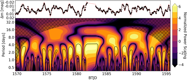
Figure 8. Top: 2 minute sampled TESS lightcurve of WR24 binned to have one data point per hour. The red dashed line is the result of the inverse wavelet transform of the wavelet analysis performed using the Mexican-hat mother function on the signal. Bottom: the power-spectrum of the wavelet analysis. The hashed region corresponds to the cone of influence of the period of the wavelets. The large, relatively uniform feature observed around T = 1582 days corresponds to the lack of data as seen in the lightcurve. The contour lines enclose regions with greater than 95% confidence for the red-noise component.
Download figure:
Standard image High-resolution image4. Discussion
In view of the trend we have found between the typical amplitude of stochastic variability characterized by the α0 parameter and the wind terminal velocity, and also considering the six other observed correlations, we discuss in this section the various physical processes that could conceivably lead to stochastic variability in WR winds. Note that a similar correlation was found between the stellar temperature, T*, and the spectroscopic variability of WR-star wind lines by Chené et al. (2020), indicating that hotter stars show a smaller level of variation than cooler stars. As the continuum is thought to be formed at the outer boundary of the dense wind (τ = 2/3) for WR stars, this result is not surprising.
4.1. Line Deshadowing Instability
As the LDI is normally assumed to be intrinsic to the driving of hot-star winds, could this process alone explain the observed photometric variability we found in WR stars? And, if not, can we determine if the LDI contributes significantly to the variability?
Sundqvist et al. (2018) have shown that for a wind with a velocity structure described by a beta velocity law, the LDI produces clump sizes of the order of the Sobolev length,  . Note that although here the thermal speed is related to the wind temperature and not the stellar temperature, stellar and wind temperatures are correlated. Since the thermal speed is expected to be about 1% of the terminal speed, this process is expected to lead only to very small clumps, according to the above equation. It is far from clear if such small structures can lead to the level of photometric variability we see in WR winds.
On the other hand, if WR winds are self-similar, a more appropriate parameter to consider would then be LSob/R*, which is proportional to the square root of the wind temperature divided by the terminal velocity. As faster winds are known to be hotter (Sander et al. 2019), it is possible, if the correlation between v∞ and T* is steeper than the square root, that the Sobolev length inversely correlates with the temperature, i.e., hotter winds have smaller Sobolev length and therefore potentially smaller wind structures. This in turn can lead to a lower level of variability as larger clumps are expected to scatter more flux, and while a high number of smaller clumps can possibly scatter the same amount of flux, they would need to occupy a larger portion of the surrounding area of the WR disk to do so, a configuration we think is less likely to happen than single, larger clumps doing the scattering.
In order to check that increasing clump size directly leads to increased variability, we used the same simple clumping model as presented in Ramiaramanantsoa et al. (2019). These authors where able to produce similar lightcurves to that observed with BRITE for the WN8h star WR40 by populating its wind with a distribution of clumps and calculating the resulting continuum light that is Thomson scattered off these clumps as they travel through the wind. The f parameter in this model sets the percentage of incoming stellar flux that is Thomson scattered by the biggest clump. Smaller clumps scatter less flux, with their size following a negative-index power law with exponent −2/3. Using increasing values of f to simulate the increasing clump size, multiple synthetic lightcurves were produced and their amplitude spectra were extracted. Following the same recipe as with our sample stars, our artificial lightcurves were then fitted with the semi-Lorentzian distribution previously shown. Figure 9 shows the fitted amplitude of variability plotted against the various f values used.
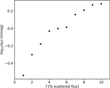
Figure 9. Amplitude of variability parameter, α0, vs. the percentage of scattered starlight for the biggest simulated clump, f.
Download figure:
Standard image High-resolution imageA clear positive trend appears, showing that, according to this simple model, stars with bigger clumps in their winds are expected to show an increased amplitude of variability in their amplitude spectrum, similar to the observed trend.
In Figure 10 we present the values found in our simulations for the steepness parameter of the red component of the stochastic variability, γ, as a function of various model parameters: f; the lifetime of clumps, T; the mass-loss rate,  the stellar radius, R*; and the exponent of the size distribution,
  . Although no obvious correlation is found, we note that all the lightcurves produced by the model have an associated γ value in the range 1.5 < γ < 3.0, with the exception of simulations with a clump lifetime parameter T below 2 hr, for which the range becomes 3.5 < γ < 5.0. As can be seem from Figures 6 and 7, this partly overlaps with most of the γ values determined from our data sets, which are concentrated in the range 0.8 < γ < 3.0, with a smaller number with γ > 3.0.

Figure 10. Steepness of the amplitude spectrum, γ, as a function of various model parameters of the scattering of stellar light on clumps in the wind and vs. the mass-loss rate and stellar radius.
Download figure:
Standard image High-resolution image
Krtička & Feldmeier (2018, 2021) have recently suggested that variable wind blanketing that results in extra heating of the stellar photosphere can explain the stochastic variability in optically thin winds of O stars. Indeed, a variable mass-loss rate caused by LDI can in turn produce detectable light variability at the photosphere of the order of tens of millimagnitudes. Although for WR stars this effect is unlikely to contribute directly to the photometric variability since the stellar surface is hidden by the optically thick stellar outflow, it might propagate in the wind and contribute somehow to the wind variability in the observable parts of the wind.
Therefore, there are several arguments in favor of LDI playing an important role in generating the observed stochastic photometric variability. LDI could even lead to an anticorrelation between the level of the photometric and spectroscopic stochastic variability, as observed in the winds of WR stars, with hotter winds having smaller clumps, leading to a lower amplitude of variability. However, this does not exclude that an additional process occurring at the stellar surface could seed the instabilities and affect the clump characteristics in the winds. In the next two sections, we discuss two such possible processes.
4.2. Subsurface Convection Zones
Following the original work of Cantiello et al. (2009) on the effects of subsurface convection zones caused by an FeCZ on the optically thin winds of OB stars, Grassitelli et al. (2016) studied the effects of this convective zone on the radiative envelopes of WR stars in the 2–17 M⊙ mass range. Although only small-amplitude (∼1 km s−1) total velocity perturbations were found for lower-mass stars, they found that for masses larger than ∼10 M⊙, surface convective velocities of the order of 10 km s−1 were expected. More precisely, they predicted a linear increase in convective velocities with stellar mass from 2 to 26 km s−1, approaching the local sound speed for the higher masses. Although these turbulent surface velocity fields are predicted to be somewhat attenuated in the radiative zones above the FeCZ, the predicted surface total velocities, vsurf, are of the same order of magnitude as the convective velocities and are predicted to follow the same increase with mass. These predictions are supported by observations of stochastic spectroscopic variations of the winds of WN stars, quantified by the rms of the line flux relative to the continuum, that are found to show an increase in amplitude with increasing mass (see their Figure 10).
The range of dominant frequencies of the variability (νchar) can help shed more light on the physical mechanism behind the observed variability. FeCZ are expected to have a typical turnover frequency of 6–60 μHz (0.5–5 day−1) (Cantiello et al. 2009; Cantiello & Braithwaite 2011, 2019), which can be transmitted to the above radiative layer since it is below the Brunt–Väisälä frequency of 0.1–1 mHz (Cantiello et al. 2009). As shown in Figures 6 and 7, almost all the stars in our sample have a characteristic frequency in this expected range. However, the typical timescale associated with convection determined for helium stars, 102–103 s (Grassitelli et al. 2016) is some two orders of magnitude shorter, leading to much higher characteristic frequencies of  . This does not agree with our observed values.
The temperature of the outer hydrostatic layers of OB and WR stars is expected to be an important parameter in the surface variability produced by the FeCZ (Cantiello et al. 2009; Grassitelli et al. 2015) because it has a direct influence on the location of the FeCZ caused by the partial ionization of Fe-peak elements at  . For higher temperatures, the FeCZ will be located closer to the surface, and therefore the observed photometric variability will be reduced because the convective mass flux perturbing the base of the wind will be smaller. This effect could play a role in explaining the origin of the possible trend we find in our sample between the amplitude of photometric variability and the stellar temperature, Teff, if confirmed (see Figures 6 and 7). This supports the idea that a subsurface convection zone can directly influence the formation of clumps in the winds of WR stars, particularly for stars above a mass of ∼10 M⊙.
4.3. Core-generated Gravity Waves
Another possible source of variability in hot, massive stars that has been put forward in the recent literature is a large number of IGWs, excited by turbulent convection at the interface of the convective core and the radiative zone lying above it (Aerts & Rogers 2015; Bowman et al. 2019a, 2020). IGWs have been claimed to be one possible source of waves that can produce the velocity field required to generate the ubiquitous macroturbulent broadening that characterizes the absorption lines of many OB stars, with the presence of a subsurface convection zone being another (e.g., Aerts & Rogers 2015). In support of this interpretation, a strong correlation was found between the surface macroturbulent speed and the amplitude of stochastic variability in OB stars; see Bowman et al. (2020), who also showed that IGWs become increasingly important in stars with larger spectroscopic masses and luminosities. Note, however, that in order to avoid numerical instabilities, the thermal diffusivity must be increased in those models, and as a consequence the heat flux must be artificially increased to compensate for the resulting damping (e.g., Rogers et al. 2013; Aerts & Rogers 2015). Other authors also claim that the observed photometric variability of OB stars is incompatible with the predicted signature (e.g., Shiode et al. 2013; Lecoanet et al. 2019). As WR stars are among the most luminous stars, IGWs could potentially play a role in their internal structure, as well. However, contrary to massive MS stars, we do not see the surface of WR stars directly, and therefore we can only see these perturbations if they propagate outward in the wind. For the optically thin wind of the O9.5 supergiant star HD188209, Aerts et al. (2017) have shown that perturbations formed at the stellar surface do indeed seem to propagate in the wind. Similarly, this was also demonstrated for the B1 Iab supergiant ρ Leo (Aerts et al. 2018). It remains to be shown what happens in the optically thick winds of WR stars.
The steepness of the amplitude spectrum of the stochastic photometric variability (characterized by the γ exponent) can also help shed some light on the cause of the stochastic variability. Recent three-dimensional simulations by Edelmann et al. (2019) predict that IGWs are compatible with a steepness of amplitude exponent 0.8 < γ < 3.0, with the value also depending on the rotation rate and evolutionary stage of the star (Ratnasingam et al. 2020). As can be seen from Figures 6 and 7, we find that the vast majority of WR stars in our sample have a γ exponent in that range.
5. Conclusions
In this paper we have presented an analysis of the stochastic photometric variability of 50 Galactic WR stars using 122 lightcurves obtained with the BRITE-Constellation, TESS and MOST satellites. We calculated the discrete Fourier transform of all the lightcurves and fitted the amplitude spectrum with a semi-Lorentzian profile representing a combination of white and red noise. We searched for correlations of the fitted parameters with wind and stellar parameters in an attempt to shed new light on the physical processes responsible for the stochastic variability.
We found a significant correlation between the level of photometric variability and the terminal velocity of the wind. As terminal wind speed and stellar temperature are related, this is reminiscent of the correlation between the level of spectroscopic variability, characterized by the rms of the flux level in wind lines relative to the neighboring continuum for series of spectra and temperature found in previous publications (e.g., Chené et al. 2020). For WNh stars specifically, we also found correlations between the level of variability and stellar temperature and also between the characteristic frequency of the variations and both the terminal speed of the wind and stellar temperature. For classical WR stars with hydrogen-free winds, we found negative correlations between the level of variability and both the mass-loss rate and bolometric luminosity. We also observed that stars that were observed more than once show significant changes in the photometric variability amplitude, characteristic frequency of the variations, and steepness of the amplitude spectrum from one observing run to the next, even with data from the same satellite. Furthermore, we find that the vast majority of observed characteristic frequencies for the variations lie between  and that the values of the steepness of the amplitude spectrum are generally found to be in the range
  .
.
We discuss three nonmutually exclusive physical processes that may be responsible for the stochastic photometric variability. The line deshadowing instability is found to be a plausible process, but we do not exclude that either a subsurface convection zone and/or internal gravity waves can contribute to an increased level of variability.
We conclude that although arguments in favor of either of these three physical processes can be made to reproduce the characteristics of the observed variability of WR stars, we have found no definite evidence in favor of one or the other. It is very possible that all will eventually be found to contribute in some way either directly to the photometric variability or indirectly to the clumping in the wind that in turn may have a definite impact on the variability.
We would first like to thank our referee, Luca Grassitelli, for an excellent report on the first version of this paper. His careful analysis of our work and insightful comments allowed us to greatly improve the quality and significance of the presented research results. We would like to thank Dominic Bowman for stimulating discussions and sound advice on the pulsation properties of massive stars, Fourier analysis, and TESS data reduction. N.S.L. and A.F.J.M. wish to thank the Natural Sciences and Engineering Council (NSERC) of Canada for financial support. G.H. thanks the Polish National Center for Science (NCN) for support through grant No. 2015/18/A/ST9/00578. K.Z. acknowledges support by the Austrian Space Application Programme (ASAP) of the Austrian Research Promotion Agency (FFG). A.P. was responsible for image processing and automation of photometric routines for the data acquisition by the BRITE-nanosatellite constellation, and was supported by SUT Rector's grant Nos. 02/140/SDU/10-22-01 and 02/140/RGJ21/0012. Wavelet software was provided by C. Torrence and G. Compo, and is available at URL: http://atoc.colorado.edu/research/wavelets/.
Data Availability
The detrended BRITE, MOST, and TESS data used in this study, as well as images of the lightcurves and of the periodograms fitted with the semi-Lorentzian model, are available on Figshare, at https://dx.doi.org/10.6084/m9.figshare.13827530.
Footnotes
- 10
- 11
Excluding the factor of two between the electron temperature with respect to the temperature at an optical depth of 20.