


Abstract
In preparation for deep extragalactic imaging with the James Webb Space Telescope, we explore the clustering of massive halos at z = 8 and 10 using a large N-body simulation. We find that halos with masses of 109–1011 h−1 M⊙, which are those expected to host galaxies detectable with JWST, are highly clustered with bias factors ranging from 5 to 30 depending strongly on mass, as well as on redshift and scale. This results in correlation lengths of 5–10 h−1 Mpc, similar to those of today's galaxies. Our results are based on a simulation of 130 billion particles in a box of size 250 h−1 Mpc using our new high-accuracy Abacus simulation code, the corrections to cosmological initial conditions of Garrison et al., and the Planck 2015 cosmology. We use variations between sub-volumes to estimate the detectability of the clustering. Because of the very strong interhalo clustering, we find that a medium-sized survey with a transverse size of the order of 25 h−1 comoving Mpc (about 13') may be able to detect the clustering of z = 8–10 galaxies with only 500–1000 survey objects if the galaxies indeed occupy the most massive dark matter halos.
Export citation and abstract BibTeX RIS
1. Introduction
Galaxy formation is strongly influenced by large-scale structure. In dark matter halos of high mass, effects of supernova feedback are less dominant, easing the formation of stars and galaxies out of gas. Halos hosting luminous galaxies at high redshift are expected to be massive, rare, and therefore highly clustered. This in turn implies that the galaxies should be highly clustered, corresponding to large bias values (Kauffmann et al. 1999; Jose et al. 2017). Observations of Lyα emitters (Takada et al. 2014; Sobacchi & Mesinger 2015; Cai et al. 2017; Ouchi et al. 2018), Lyα blobs (Nilsson et al. 2006; Yang et al. 2009, 2010), and Lyman-break galaxies (Barone-Nugent et al. 2014; Harikane et al. 2016, 2018) and deep field observations with the Hubble Space Telescope (HST; Overzier et al. 2006; Schenker et al. 2013; Robertson et al. 2014) have supported this, finding large angular clustering and field-to-field density variations.
As massive halos are extreme fluctuations in the density field, the resulting number of these host sites and their clustering is unusually sensitive to the cosmological model. Therefore, measuring the clustering can be indicative of the halo mass function. This has been a common application of halo occupation distribution (HOD) modeling, a method in which the association of galaxies to halos of a given mass leads to detailed predictions of galaxy clustering (for a review, see Cooray & Sheth 2002).
However, the extreme sensitivity of the clustering to the cosmological properties also requires careful control of the initial conditions and numerical methods. In this paper, we present a large-scale high-resolution N-body simulation to investigate halo clustering at high redshifts. Our work includes several improvements that we argue will improve the reliability of the results. First, we adopt our cosmological parameters from the most recent Planck measurements (Planck Collaboration et al. 2016). The increase in the matter density, Ωmh2, relative to previous results from the cosmic microwave background increases the small-scale fluctuations in the cold dark matter model and hence the abundance of halos at a given mass. Second, we utilize our new N-body cosmological code Abacus, which features high force accuracy. We adopt a small particle mass of 107 h−1 M⊙ so that halos of 1010 h−1 M⊙, which we expect will be typical of detectable galaxies with JWST, will be well resolved. The high speed of Abacus allows us to still run a box of 130 billion particles filling 248.8 h−1 Mpc, big enough to capture most of the large-scale modes relevant to the formation of these halos. Third, we utilize the corrections to the linear-theory initial conditions highlighted by Garrison et al. (2016) and also use the methods in that paper to include terms from second-order perturbation theory in the initial conditions.
In order to compare with upcoming James Webb Space Telescope (JWST) deep field surveys at high redshifts (Cowley et al. 2018; Williams et al. 2018), we analyze time slices of our simulation at z = 10 and z = 8. Since the simulation volume of around (250 h−1 Mpc)2 is much larger than the volume of a typical JWST survey, we are able to cut the simulation into many sub-volumes and use the variations between them to estimate the covariance of the clustering. Here, we choose to divide the region into 10 × 10 boxes, investigate the clustering in our simulated halo catalogs, and predict a detection significance for one box representing a single survey. These boxes correspond to about 170 square arcminutes, somewhat smaller than the JADES survey described in Williams et al. (2018) and well within the capabilities of JWST.
While we were preparing this publication, the work of Bhowmick et al. (2018) was published, which investigated clustering at z > 7 using a cosmological hydrodynamical simulation called the BLUETIDES simulation (Feng et al. 2016). Their research obtained results that are compatible with ours.
In Section 2, we introduce the simulation used in this work. In Section 3, we describe our methodology and then present our results. In Section 4, we give our conclusion and a discussion.
2. Cosmological Simulation
Abacus is a code for cosmological N-body simulation (Garrison et al. 2019) that is both extremely fast and highly accurate, aided by recent computational techniques and commodity hardware for high performance computing. Abacus utilizes a novel, fully disjoint split between the near-field and far-field gravitational sources, solving the former on GPU hardware and the latter with a variant of a multipole method. The result is very high speed, in excess of 20 million particle updates per second on a single 24-core workstation. Further, Abacus is built to store most of its data on a high-speed disk system, allowing us to run multi-terabyte problems on a single computer with only modest amounts of RAM.
In this paper, we use a single 51203 particle simulation of a (248.8 h−1 Mpc)3 box. This results in a particle mass of 107 h−1 M⊙, suitable to robustly identify halos with masses around 1010 h−1 M⊙. We evolve the simulation using a standard leapfrog integration with 225 time steps from z = 199 to z = 10 and 67 more to z = 8. All particles have the same time step. The simulation was run on a single commodity-based 24-core dual Xeon workstation with 256 GB of RAM, two NVidia GeForce GTX 980 Ti GPUs, and a RAID system providing over 1.5 GB s−1 of disk speed, with each time step taking about 2.2 hr.
Marcos et al. (2006) showed that solutions to the discrete N-body problem do not correctly recover the continuum linear perturbation theory found in cosmological textbooks for wavenumbers near the Nyquist wavenumber. Most Fourier modes grow too slowly, although a few grow too quickly. While the effects are small for modes much larger than the interparticle spacing, we are nevertheless concerned that the formation of extreme halos is very sensitive to small changes in perturbation amplitude.
We therefore use the initial conditions proposed by Garrison et al. (2016), whose method seeks to cancel out these linear-theory errors at a given target redshift (here chosen to be z = 49). This method is careful to use only the longitudinal linear-theory growing mode, which differs from the wavevector in the discrete theory. It then adjusts the initial displacement amplitudes of each mode so as to compensate for the non-standard growth function that will be encountered between the initial redshift of z = 199 and the target redshift. Finally, we include second-order effects on the initial perturbations by inverting the particle displacements and using the sum of the forces in both cases to isolate the second-order forces, which are then applied as displacements and velocities assuming the continuum limit. Such second-order corrections are known to be important for the formation of the most massive halos (Crocce et al. 2006; Sissom 2015).
We adopted the cosmology of Ωm = 0.31415, ΩDE = 1 − Ωm, ΩK = 0, h = 0.6726, σ8 = 0.83, and Nspec = 0.9652 from the Planck measurements (Planck Collaboration et al. 2014). The linear power spectrum was calculated using the package "Code for Anisotropies in the Microwave Background" (Lewis et al. 2000). We started at the initial redshift of z = 199 and used the output time slice at z = 10 and 8.
The group-finding algorithm that we adopt is the friends-of-friends algorithm (Huchra & Geller 1982; Press & Davis 1982), which connects all pairs of particles within a certain critical distance and then identifies clumps of interconnected particles above a certain multiplicity threshold as a halo. As our goal is to establish a more robust prediction of halo abundance and clustering, we require at least 300 particles in a halo and focus on the case of 1000 particles (1010 h−1 M⊙) and at a redshift of z = 10 as our fiducial case. This ensures that halos are robustly found. For example, Garrison et al. (2016) found that such multiplicity yielded well-converged results with respect to particle discreteness when using the initial conditions developed in that work.
We make the halo catalogs from our simulation available at http://nbody.rc.fas.harvard.edu/public/JWST_products/. Further documentation of the data files is given in Garrison et al. (2018) and at https://lgarrison.github.io/AbacusCosmos/.
3. Large-scale Structure of High-redshift Halos
3.1. Clustering Methodology
3.1.1. Two-point Clustering Statistics
We aim to study the clustering of halos as a function of their mass using the two-point clustering statistics: the familiar two-point correlation function (2PCF) and power spectrum. We define samples based on thresholds in halo mass and compare the results between different threshold values, as well as with the correlations of the matter field and of linear theory. It is worth noting that halos of the requisite mass are treated as containing only one galaxy. HOD models commonly assign additional satellite galaxies to the most massive halos, which can further increase the clustering strength, particularly at intrahalo separations but also at interhalo separations.
For our analysis of the halo clustering, we split the simulation volume into 100 rectangular pieces, each 25 by 25 by 250 h−1 comoving Mpc. We introduce the sub-volumes so that we can use the dispersion among them to determine the covariance matrix of the 2PCF. However, it is also the case that these volumes correspond to roughly the scale of a substantial JWST survey, about 13' wide and Δz = 2 at these redshifts.
We compute the 2PCF in each sub-volume, ignoring any periodicity, using the estimator of Landy & Szalay (1993):

where DD, DR, and RR indicate the counts in each separation bin of data–data, data–random, and random–random halo pairs, respectively. The random catalog is a uniform distribution across the entire volume. In detail, we use the simplicity of the rectangular volume to accelerate the DR and RR calculations near the boundaries by evaluating the truncated spherical volume as a function of the distances to boundaries at a variety of reference points and then interpolating. We confirm that the mean of the sub-volume results is very similar, save at the largest separations, to the result for the full periodic simulation volume, where the DR and RR counts are trivially computed in the limit of infinite sampling.
For the correlations of the nonlinear matter field and linear theory, we first obtain their power spectra and then compute the 2PCFs from the power spectra based on the inverse Fourier transform relation described in Equation (2), where Σ = 0.10 h−1 Mpc is a smoothing constant to guarantee the convergence of the numerical integration in the Fourier transformation.

The power spectra of the halos and of the matter field have been calculated in the conventional way using Fourier transforms of a large periodic gridded representation of the density field. Shot noise is removed as presented in Bianchi et al. (2015) and we divide by the transfer function corresponding to triangular-shaped assignment so as to reconstruct the original power spectrum from the alias summation (Jing 2005).
3.1.2. Detection Significance
Based on the 2PCFs of the 100 sub-volumes, the (j, k) entry of the covariance matrix C is given by
where dij denotes the jth separation bin of the 2PCF in the ith sub-volume. We then compute the detection significance from
where  . We use dobs,i = 0 to correspond to the unclustered case, which we interpret as a non-detection.
3.2. Results
3.2.1. Overview of the Halo Sample
We begin in Figure 1 with the mass distribution of our halo samples at z = 10 and z = 8, obtained by the friends-of-friends algorithm. The numbers of halos above a series of mass cuts are available in Tables 1 and 2. Below we primarily use the case of low particle number cut Nmin = 1000 as an illustration.
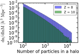
Figure 1. A histogram of comoving number density of halos in bins of halo particle multiplicity. We divide the halo counts by the logarithmic bin width to yield the comoving number density per logarithmic mass bin. Recall that each particle is 107 h−1 M⊙. The two histograms at z = 10 and z = 8 are overplotted.
Download figure:
Standard image High-resolution imageTable 1. Effects of Changing the Particle Number Cut Value for z = 10 Halos
| Nmin | Mmin | Number | ξ(r) | w(R) | P(k) (h−3 Mpc3) |

|

|
Ndet | ||||
|---|---|---|---|---|---|---|---|---|---|---|---|---|
| (109 h−1 M⊙) | of Halos | 1 h−1 Mpc | 5 h−1 Mpc | 1 h−1 Mpc | 5 h−1 Mpc | 0.1 h Mpc−1 | 1 h Mpc−1 | 3D | 2D | |||
| 300 | 3.0 | 296364 | 10.9 | 0.85 | 0.19 | 0.060 | 1996 | 185 | 85 | 52 | 872 | 1425 |
| 450 | 4.5 | 138720 | 15.2 | 1.04 | 0.25 | 0.070 | 2468 | 257 | 51 | 27 | 680 | 1284 |
| 700 | 7.0 | 57127 | 22.5 | 1.31 | 0.35 | 0.087 | 3190 | 380 | 27 | 20 | 529 | 714 |
| 1000 | 10.0 | 26864 | 32.4 | 1.61 | 0.45 | 0.106 | 3976 | 536 | 19 | 15 | 353 | 448 |
| 1500 | 15.0 | 10668 | 52.4 | 2.02 | 0.64 | 0.130 | 5250 | 863 | 10 | 8 | 267 | 333 |
| 2000 | 20.0 | 5341 | 76.6 | 2.34 | 0.88 | 0.149 | 6283 | 1246 | 5 | 4 | 267 | 334 |
| Matter Density Field | 8.25 × 10⁻² | 1.43 × 10⁻² | ⋯ | ⋯ | 83.3 | 1.017 | ⋯ | ⋯ | ⋯ | ⋯ | ||
| Linear Theory | 7.04 × 10⁻² | 1.36 × 10⁻² | ⋯ | ⋯ | 77.8 | 0.931 | ⋯ | ⋯ | ⋯ | ⋯ | ||
Note. For each Nmin, we examine the number of halos in our sample, the 3D and 2D 2PCFs at two representative distances, the power spectra at two representative lengths of wavevectors, and the 3D and 2D χ2 detection significance for a 1% sub-volume of our simulation. The quantity Ndet in the last two columns is the number of galaxies required to reach a detection significance of χ2 = 25 assuming that the galaxies occupy the most massive halos. This is given for the 3D and 2D cases and is computed from the previous columns as (25/χ2)(Nhalo/100).
Download table as: ASCIITypeset image
Table 2. Same as Table 1, but at Redshift z = 8
| Nmin | Mmin | Number | ξ(r) | w(R) | P(k) (h−3 Mpc3) |

|

|
Ndet | ||||
|---|---|---|---|---|---|---|---|---|---|---|---|---|
| (109 h−1 M⊙) | of Halos | 1 h−1 Mpc | 5 h−1 Mpc | 1 h−1 Mpc | 5 h−1 Mpc | 0.1 h Mpc−1 | 1 h Mpc−1 | 3D | 2D | |||
| 300 | 3.0 | 1916736 | 4.8 | 0.53 | 0.11 | 0.043 | 1201 | 84 | 199 | 105 | 2408 | 4564 |
| 450 | 4.5 | 1038761 | 6.0 | 0.62 | 0.13 | 0.047 | 1412 | 106 | 160 | 117 | 1623 | 2220 |
| 700 | 7.0 | 515064 | 8.0 | 0.74 | 0.16 | 0.055 | 1703 | 139 | 119 | 62 | 1082 | 2077 |
| 1000 | 10.0 | 284623 | 10.3 | 0.86 | 0.19 | 0.061 | 2003 | 178 | 99 | 50 | 719 | 1423 |
| 1500 | 15.0 | 140220 | 14.3 | 1.07 | 0.24 | 0.069 | 2488 | 243 | 63 | 38 | 556 | 923 |
| 2000 | 20.0 | 82914 | 18.3 | 1.23 | 0.30 | 0.077 | 2913 | 309 | 48 | 26 | 432 | 797 |
| 3000 | 30.0 | 38051 | 27.3 | 1.55 | 0.42 | 0.097 | 3720 | 455 | 27 | 17 | 352 | 560 |
| 4000 | 40.0 | 21267 | 37.6 | 1.83 | 0.52 | 0.114 | 4535 | 628 | 15 | 10 | 354 | 532 |
| 6000 | 60.0 | 8894 | 59.9 | 2.46 | 0.76 | 0.162 | 6184 | 972 | 9 | 6 | 247 | 371 |
| 8000 | 80.0 | 4678 | 84.3 | 3.02 | 1.02 | 0.189 | 8028 | 1392 | 6 | 3 | 195 | 390 |
| Matter Density Field | 0.127 | 2.10 × 10⁻² | ⋯ | ⋯ | 113 | 1.58 | ⋯ | ⋯ | ⋯ | ⋯ | ||
| Linear Theory | 0.105 | 2.03 × 10⁻² | ⋯ | ⋯ | 116 | 1.39 | ⋯ | ⋯ | ⋯ | ⋯ | ||
Note. The maximum of the low-mass cutoff is extended to 8 × 10¹⁰ h−1 M⊙ so that the sample size of the most massive halos sample remains around 5000.
Download table as: ASCIITypeset image
Figure 2 shows a 25 h−1 Mpc thick slice of our simulation at z = 10, the thickness chosen to match the width of one of our sub-volumes. The shaded region shows the same width, which allows one to gauge survey-to-survey variations by eye. One can see that there will indeed be such variations, depending on the chance intersection of the survey pencil beam with clusters and voids.

Figure 2. A thin slice through the simulation box showing halos larger than 300 particles (3 × 10⁹ h−1 M⊙) at z = 10. Each halo is plotted as a circle with radius proportional to the 90th percentile of the radial particle distribution ("r90"); the radii are inflated by a factor of 10 for plotting purposes. We imagine this slice as a side-on view of what an observer to the left of the box would see; thus, the horizontal axis is redshift and the vertical axis is angular position. The depth of the slice is 25 h−1 comoving Mpc, or 13 2, which is the size of one of our "sub-volumes." The horizontal shaded region demarcates the same width.
Download figure:
Standard image High-resolution image3.2.2. Clustering in 3D Real Space: Halos, Matter Field, and Linear Theory
Following the methods presented in Section 3.1.1, we compute the 2PCF of the z = 10 halos containing more than N = 1000 particles and show the result in Figure 3 along with the 2PCF of the z = 10 matter field and linear theory. We adopt the case Nmin = 1000, Mmin = 1010 h−1 M⊙ as our representative one. This corresponds to 270 objects in a 13' × 13' region at z = 10. To remove the steep scale dependence of the 2PCF, we choose to plot the expression r2ξ(r) in the upper panel of Figure 3. This choice is common in the low-redshift literature. As we can see, the matter-field 2PCF is consistent with the prediction of the linear theory, while the halo 2PCF is larger by a factor of the order of 102–103, corresponding to clustering biases of 10–30.

Figure 3. Comparison of the matter 2PCF (green), the halo 2PCF (blue), and the 2PCF predicted by linear theory at z = 10 (red) for halos containing more than 1000 particles in a 1% sub-field, in r2ξ(r) (upper panel) and ξ(r)/ξref(r) (lower panel). Note that the error bars in both cases indicate the standard deviation of a 1% sub-volume in our 10 × 10 partitioning (not the error on the mean for the full simulation volume). The y axis is in r2ξ(r) in the upper panel, where the flat profile of the halo 2PCF indicates the r−2 power-law relationship. In the lower panel, we can see that the matter power spectrum is basically consistent with the prediction of linear theory, except for the distances below the grid scale where the matter 2PCF gets larger by a factor of 4. The halo 2PCF is highly biased by a multiple of 2 × 10² to 2 × 10³.
Download figure:
Standard image High-resolution imageTo highlight the scale-dependent bias, we repeat these results in the lower panel of Figure 3 after dividing by the linear-theory correlation function. This shows a notable increase in bias at scales below 2 h−1 Mpc compared to a possible plateau at large scale. We stress that the comoving diameter of a 1010 h−1 M⊙ halo is about 50 h−1 kpc, so this scale dependence in the bias is occurring well outside the halo scale and indeed beyond even the 300 h−1 kpc scale of the initial Lagrangian volume corresponding to this mass. We further note that this scale dependence occurs even though we have omitted satellite galaxies from our analysis. Indeed, because two halos cannot be closer together than the sum of their radii, our 2PCF drops precipitously at small scales. We do not plot results interior to 0.3 h−1 Mpc so as to comfortably avoid this effect.
We then computed the corresponding power spectra for the three cases. These are shown in Figure 4, with the linear-theory power spectrum being the reference. Again, we obtain a qualitatively similar result to the previous plot (Figure 3).

Figure 4. Comparison of the matter power spectrum (green), the halo power spectrum (blue), and the power spectrum predicted by linear theory at z = 10 (red, taken as reference). The matter power spectrum is very consistent with the prediction of linear theory. The halo power spectrum, however, has a very high bias of the order of 102–103.
Download figure:
Standard image High-resolution imageFinally we investigate the dependence of the 2PCF on the halo mass cut. In Figures 5 and 6, we plot r2ξ(r) at z = 10 and z = 8, respectively, for a range of halo mass cuts (3, 4.5, 7, 10, 15, 20 × 109 h−1 M⊙ for both cases, and additionally 30, 40, 60, 80 × 109 h−1 M⊙ for z = 8). In Figure 5, we find a very strong increase in bias with increasing mass cut. Further, the correlation functions are shallower than r−2 at lower masses, but steeper than r−2 at higher masses. Again, this increase is occurring even though we have not included any satellite galaxies in our catalogs and it involves scales beyond the virialized diameters of the halos.
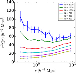
Figure 5. The 2PCFs for z = 10 halos by different mass cutoff represented by the minimum number of particles in the halo finder. For example, the curve labeled 300 shows the 2PCF for all halos that contains more than 300 particles. One can see the strong trend whereby the higher mass samples have larger 2PCF amplitudes and higher bias, i.e., more massive halos are more clustered than less massive ones. For the 2PCF of the sample with the highest mass, the shot noise in this sample of low number density is substantial. For this sample, we include the standard deviation of the mean 2PCF of our entire simulation box (not as in Figure 3 where the errors for a 1% sub-volume were plotted). The errors for the higher density samples are substantially smaller. We note that comparisons between curves are partially correlated due to both large-scale structure and the overlapping mass ranges of the halo selections. This implies that ratios between samples are more tightly constrained than the variance within a sample would suggest.
Download figure:
Standard image High-resolution image
Figure 6. The same as Figure 5, but at redshift z = 8. We extend the upper limit of the low-mass cutoff up to 8 × 10¹⁰ h−1 M⊙ so that the sample size of the most massive halos remains around 5000 (see Tables 1 and 2).
Download figure:
Standard image High-resolution imageFigure 6 shows the same progression at z = 8. The clustering amplitudes at fixed mass are smaller at low redshift, indicating that the clustering bias is falling faster than the growth function is increasing. However, the clustering amplitudes at fixed number density are more comparable. Tables 1 and 2 report some characteristic values of different measurements of the clustering. For the range of particle number cutoffs mentioned above, we present the various statistics, each at two representative values (1 h−1 Mpc and 5 h−1 Mpc for the 2PCF, 0.1 h Mpc−1 and 1 h Mpc−1 for power spectrum). As comparisons, we also give the corresponding 2PCFs and values of the power spectrum obtained from the matter density field and linear theory instead of halos. Computing the square root of the ratio of the two 2PCFs indicates a bias factor ranging from 5 to 30.
3.2.3. Halos Clustering in the Projected 2D Sky Plane
In many imaging surveys, our knowledge of the line-of-sight position of galaxies would be limited to the precision of photometric redshifts. Our measurement of small-scale clustering will then rely on the angular distribution, with the photometric redshifts used to bound the projection effects. To approximate this situation in our simulation, we project all of the coordinates onto the sky plane by assigning a uniform value to the x coordinate, which is in the redshift direction. We label the resulting correlation function as w(r), the 2D 2PCF. Given the 250 h−1 comoving Mpc depth of our box, this corresponds at these redshifts to a projection of about Δz = 2, which is typical of photometric redshift accuracy in Lyman-break samples. We investigate the dependence of the 2D 2PCF on the value of the mass cut. The result is shown in Figure 7, which is analogous to Figure 5 in 3D real space. This time we plot the function rw(r), equivalent to an r−2 power-law slope of the correlation function. The stratified structure showing an increasing bias with higher halo mass cut is similar to its 3D counterpart shown in Figure 5. We adopted a simple redshift slice in this paper, but in a real survey there would be some smoothly peaked redshift distribution n(z). Converting between spatial and angular clustering by the Limber formula (Limber 1953) indicates that the amplitude of clustering scales as the integral n(z)2. Detailed interpretation of the clustering amplitude requires knowledge of n(z). Of particular concern are interlopers from much lower redshift, where the angular scale corresponds to a smaller physical scale and hence more intrinsic correlations. Such contributions are suppressed as the square of the contamination rate, so moderately pure samples can reduce this uncertainty dramatically.
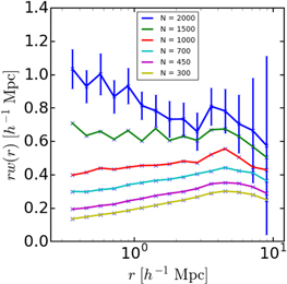
Figure 7. The same as Figure 5, except that this plot shows the 2D 2PCF (projected onto the sky plane) for the corresponding cutoffs in halo particle number.
Download figure:
Standard image High-resolution image3.2.4. Halos Clustering in 3D Redshift Space
With precise spectroscopic redshifts, one can make more accurate clustering measurements. In this case, one must contend with the redshift-space distortions caused by peculiar velocities. Figure 8 shows the 2PCFs in real space and in redshift space for the Nmin = 1000 halos at z = 10. The distorted 2PCF gives lower correlation on smaller scales and higher correlation on larger scales. This is expected from the effects of small-scale peculiar velocities, which tend to make nearby objects appear further apart. We note that we have only considered the central galaxies in these massive halos. If we had included satellite galaxies in some halos, the small-scale redshift-space distortions would have been yet larger.
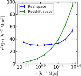
Figure 8. The redshift-space 2PCF at z = 10 for Nmin = 1000 halos compared with the real-space 2PCF of the same sample. Redshift-space distortions caused by the peculiar velocities of the halo centers of mass bring about a substantial decrease in clustering at small separations and an enhancement at large separations. The error bars are the standard deviations of the mean 2PCFs for the full simulation volume in each case, indicating that the effect of redshift-space distortion will significantly affect our detection.
Download figure:
Standard image High-resolution image3.3. Detectability
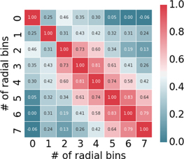
We calculate the detectability of these 2PCFs based on the covariance matrix derived from the 100 2PCFs corresponding to our 100 sub-volumes. The (i, j)th entry of the covariance matrix here is defined as the correlation of ith and jth separation bins in the 2PCF over the 100 sub-volumes; see Equation (3). The off-diagonal entries are the correlations between two different bins, and the diagonal entries are just variations of each separation bin. We use eight bins of radial separation, so as to limit the biases that result from inverting a noisy estimate of the covariance matrix (Percival et al. 2014).
In Figure 9, we plot an example of the reduced covariance matrix, defined as  . From the plot, we see higher correlations for closer bins, decaying for bins with progressively greater separation. If the variation only consists of Poisson shot noise, then we would expect the variation in each separation bin to be uncorrelated, which is rejected by such a strong off-diagonal covariance. This indicates that there is indeed a substantial contribution from the sample variance of large-scale structure in our 100 sub-volumes. Repeating this with samples of different mass thresholds shows, as expected, that the correlations of sparser samples have more diagonally dominated covariances.
Figure 9. The covariance matrix corresponding to the eight distance bins characterizing the fluctuation of the 2PCFs in 100 sub-volumes in Figure 3, where a halo number cutoff of Nmin = 1000 and z = 10 has been implemented. Each entry is normalized by the formula  , where
  are the normalized and raw entries of the covariance matrix, respectively. Such normalization guarantees that all of the diagonal entries will be converted to 1, and all of the off-diagonal entries to the interval [−1, 1]. From this plot we learn that the correlation tends to be larger for a closer pair of distance bins, indicating that the 2PCFs for the 100 sub-volumes are fluctuating in a smooth and positively correlated way. Note that the matrix will get closer to a diagonal matrix if we replace Nmin = 1000 with a larger number, indicating the fact that samples with higher Nmin will be more strongly influenced by shot noise, which is uncorrelated.
Download figure:
Standard image High-resolution image
We then use the covariance matrix to estimate the detectability of the 2PCF, according to Equation (4). The χ2 statistic here is equivalently the difference in χ2 between that of the measured 2PCF and a null ξ = 0 result. The interpretation of this in terms of detection significance depends on one's choice of model. If one had a fully unconstrained model, then one could claim a clustering detection only if the result was unusually large compared to a χ2 distribution with degrees of freedom equal to the number of bins. In our case with eight bins, finding χ2 ≳ 25 would be a 99% confident detection. However, it is more cosmologically interesting to investigate smooth models, which sharply limits the number of parameters. As an extreme, if one's model were simply a rescaling of the observed clustering, then one would have one degree of freedom, and the significance would be  σ. More likely, one would additionally include a power-law slope or other scale-dependent parameter. The resulting interpretations are hence model-dependent, but we suggest that χ2 of 20–25 would be good goal in designing a survey large enough for a first detection of large-scale clustering. We stress that our χ2 statistic is not guaranteed to follow the χ2 distribution, because the individual data points of the correlation function may not be Gaussian distributed, particularly if the survey correlations are affected by the presence or absence of a few extreme regions. Such effects are most easily studied in the context of fitting of specific models, but we caution that understanding the statistics of clustering will continue to drive requirements for large simulations of the highly biased density field.
Our results for both angular (2D) and spectroscopic redshift-space (3D) clustering are shown in Tables 1 and 2. Note that the χ2 values refer to a 1% sub-volume, i.e., about 13' square and Δz ≈ 2 deep, while the number of halos refers to the number in the full box. If galaxies are populating only the most massive halos, then for a given number density of detected galaxies one can scale the survey area to find the number required to yield a χ2 = 25 detection. According to the last two columns of our tables, the required number of galaxies changes relatively slowly compared to the 100-fold change in the number density of halos. Adding spectroscopy increases the detection sensitivity by removing noise from projection; however, this is more effective when the samples are denser. It is important to stress that these results utilize only scales above 300 h−1 comoving kpc, which is much larger than the virial radius of these halos. In other words, this procedure is only sensitive to interhalo clustering; an additional signal from intrahalo (or one-halo) clustering at small separations would boost the detection significance but might be less easily related to the halo mass distribution.
Hence, we find that a first detection of large-scale correlations could result from an angular survey of 500–1000 galaxies, if the galaxies are indeed populating only the most massive halos. The actual space density of JWST-detectable galaxies is of course unknown, with predictions varying considerably (e.g., Cowley et al. 2018; Tacchella et al. 2018). If the galaxies are rarer, it will require a survey with a wider area to obtain a detection. However, for a fixed total number of galaxies, the clustering is easier to detect with the rarer population, because the higher clustering amplitude outpaces the increasing shot noise.
4. Conclusions
In this paper, we have investigated the clustering of massive halos at z = 8 and 10 using a cosmological N-body simulation. We measured the 2PCFs and power spectra of the halo catalog above a range of cutoff masses and compared them with the same measures for the matter field and the prediction of linear theory, finding high values of the clustering bias, typically 10–20. We also measured the angular correlation function by making a line-of-sight projection and found consistent biases.
We then calculated the detectability of this clustering for an example JWST survey. We set its full volume to (250 h−1 Mpc)3. We divide our full simulation into 10 × 10 sub-volumes with equal size and estimate the 2PCF covariance matrix for a single sub-volume. We then measured χ2 of the mean 2PCF relative to the null clustering signal. Based on the angular correlation function at z = 10 of a sample exceeding 1010 h−1 M⊙, we derived an expectation of  = 15 relative to a null clustering signal from a sample of 270 galaxies. With spectroscopic information to remove false pairs from projection, this significance would increase to
  = 19 for the 3D redshift-space correlation function. Hence, we find that samples of 500–1000 galaxies could yield a detectable large-scale clustering signal (χ2 ≳ 25) if indeed the detected galaxies inhabit the most massive dark matter halos. If the joint distribution of galaxy luminosity (or more precisely, detectability) and halo mass has more scatter, then the typical host halo mass will decrease, as will the clustering amplitude.
These results indicate that the interhalo clustering of z ≈ 8–10 galaxies could be detectable with achievable sample sizes and that the amplitude of the clustering signal can offer some selection between hypotheses of galaxy formation. However, we caution that our results include only the effect of halo clustering. Galaxy formation may yet depend on additional effects, such as large-scale radiative feedback and reionization, which could cause additional large-scale clustering. Distinguishing such signals from those of halo clustering might be possible in the shape of the 2PCF or the signatures of higher-point correlations, but any interpretations of early clustering signals will need to include this caveat.
We next compare the clustering measurement at high redshift presented by Bhowmick et al. (2018) obtained from BLUETIDES, a hydrodynamical simulation code that incorporates physics of galaxies, with our clustering measurements from Abacus, a pure dark-matter N-body gravitational code. The BLUETIDES analysis gets a bias factor of 10.8 ± 0.7 for galaxies at z = 10, which is consistent with our measurements for dark matter halos. In addition, analyzing the results of these two papers via HOD modeling helps to constrain the galaxy–dark matter halo connection (see Section 3 in Bhowmick et al. 2018 for the detailed methods). However, our simulation is purely gravitational on dark matter halos without any assumption on smaller-scale physics about galaxies, and thus provides a more robust probe of clustering at high redshifts. Another unique feature of our paper is our focus on detectability of clustering from proposed deep field surveys at high redshift.
Our Abacus code is a robust gravitational N-body cosmology simulation code in the following senses. First, we adopted the latest cosmological parameters from the Planck mission (see, for example, Planck Collaboration et al. 2016). Second, we adopted an improved set of initial conditions as described in Garrison et al. (2016), which only takes the longitudinal wave mode, compensates for the non-standard growing factor across the simulated redshift range, and takes into account second-order effects. Therefore, our Abacus code is capable of doing simulations that properly evolve the nonlinear fluctuations.
Our investigation clearly reinforces the expectation for upcoming high-redshift surveys that there will be significant field-to-field variations in galaxy populations at z ≈ 10. But these variations come with an opportunity, that the clustering signal can be measured with surveys of moderate scope, giving a route to constrain the mass distribution of the host halos of these early galaxies.
We make the halo catalogs from our simulation available at http://nbody.rc.fas.harvard.edu/public/JWST_products/, so that the simulation can be used for additional analyses of clustering and the generation of JWST mock catalogs.
We thank Marc Metchnik and Philip Pinto for their contributions to the Abacus simulation code. D.J.E., L.H.G., and D.W.F. have been supported by grant AST-1313285 from the National Science Foundation, and D.J.E. is additionally supported as a Simons Foundation Investigator.