


Abstract
We present the Citizen Science program Active Asteroids and describe discoveries stemming from our ongoing project. Our NASA Partner program is hosted on the Zooniverse online platform and launched on 2021 August 31, with the goal of engaging the community in the search for active asteroids—asteroids with comet-like tails or comae. We also set out to identify other unusual active solar system objects, such as active Centaurs, active quasi-Hilda asteroids (QHAs), and Jupiter-family comets (JFCs). Active objects are rare in large part because they are difficult to identify, so we ask volunteers to assist us in searching for active bodies in our collection of millions of images of known minor planets. We produced these cutout images with our project pipeline that makes use of publicly available Dark Energy Camera data. Since the project launch, roughly 8300 volunteers have scrutinized some 430,000 images to great effect, which we describe in this work. In total, we have identified previously unknown activity on 15 asteroids, plus one Centaur, that were thought to be asteroidal (i.e., inactive). Of the asteroids, we classify four as active QHAs, seven as JFCs, and four as active asteroids, consisting of one main-belt comet (MBC) and three MBC candidates. We also include our findings concerning known active objects that our program facilitated, an unanticipated avenue of scientific discovery. These include discovering activity occurring during an orbital epoch for which objects were not known to be active, and the reclassification of objects based on our dynamical analyses.
Export citation and abstract BibTeX RIS

Original content from this work may be used under the terms of the Creative Commons Attribution 4.0 licence. Any further distribution of this work must maintain attribution to the author(s) and the title of the work, journal citation and DOI.
1. Introduction
In 1949 comets ceased to be the only solar system objects known to display activity when near-Earth asteroid (4015) Wilson–Harrington was observed with a pronounced tail (Cunningham 1950). In the seven intervening decades, fewer than 60 asteroids have been found to be active, a tiny fraction of the ∼1.3 million known minor planets, and the vast majority of discoveries have taken place in just the last 25 yr (see Table 1 of Chandler et al. 2018). Nevertheless, these objects have provided a wealth of knowledge (Hsieh & Jewitt 2006a; Jewitt 2012), ranging from informing us about the volatile distribution in the solar system and possible origins of terrestrial water (Hsieh & Jewitt 2006b), to further insight into astrophysical processes such as the Yarkovsky–O'Keefe–Radzievskii–Paddack (YORP) effect (e.g., (6478) Gault; Kleyna et al. 2019). Roughly half of the observed activity in apparently asteroidal bodies has been attributed to stochastic events, such as impacts (including the Double Asteroid Redirection Test, or DART, impact), with the remainder seen to be recurrently active, a characteristic potentially diagnostic of volatile sublimation. Before our program, fewer than 15 of the known active asteroids were classified as main-belt comets (MBCs), recurrently active, sublimation-driven active asteroids that orbit exclusively within the main asteroid belt (Hsieh & Jewitt 2006b).
A similar story applies to the Centaurs, bodies thought to originate in the Kuiper Belt that are now found between the orbits of Jupiter and Neptune (for a review, see Jewitt 2008). Unlike the active asteroids, the first active Centaur, 29P/Schwassmann–Wachmann 1 (Schwassmann & Wachmann 1927), was identified retroactively after Centaurs were realized as a class following the discovery of (2060) Chiron in 1977 (Kowal & Gehrels 1977). Notably, these bodies are too cold for water ice to sublimate, so other species (e.g., CO2) or processes must be involved (Jewitt 2009; Snodgrass et al. 2017; Chandler et al. 2020). As with active asteroids, few (<20) active Centaurs have been found, so finding more of these objects will significantly further our knowledge about this minor-planet population.
Another group of active objects not typically associated with comets are the active quasi-Hilda asteroids (QHAs), sometimes referred to as quasi-Hilda comets (QHCs), active quasi-Hilda objects, or active quasi-Hildas. This dynamical class shares a name with the Hilda asteroids, a small body population bound in stable 3:2 interior mean motion resonance (MMR) with Jupiter, and span a region from the outer asteroid belt to the Jupiter Trojans (Szabó et al. 2020). However, quasi-Hildas are not in true resonance with Jupiter, though their orbits are reminiscent of the Hildas when observed in the Jupiter corotating reference frame (Chandler et al. 2022), as discussed later in Section 6. Consequently, these objects are challenging to identify, with dynamical modeling requisite to confirm a quasi-Hilda orbit confidently. Roughly 3000 quasi-Hildas have been loosely identified (Toth 2006; Gil-Hutton & Garcia-Migani 2016), with fewer than ∼15 observed to be active.
All of the aforementioned classes (active asteroids, active Centaurs, and active QHAs) remain largely mysterious, with so few objects known that it is difficult to draw statistically robust conclusions about these populations. The clear remedy, then, is to find more of these objects. There are numerous astronomical archives containing vast numbers of images in which minor planets can be seen, but they have not been examined because of the overwhelming numbers involved. We set out to do this with the help of online volunteers through Citizen Science, a paradigm that simultaneously achieves outreach and scientific goals. Here, we (i) briefly introduce the Citizen Science project Active Asteroids and the underlying system that produces the images we show to volunteers, (ii) describe a broadly applicable technique we created to improve the quality of classification analyses, and (iii) present results stemming from the first 2 yr of the Active Asteroids program, including objects previously unknown to be active.
2. HARVEST: The Image Cutout Pipeline
With the goal of discovering previously unknown minor-planet cometary activity, we created a pipeline to extract small images of known minor planets from publicly available archival astronomical images; these extracted small images are interchangeably known as cutouts, thumbnails, or "subjects" in Zooniverse terminology. We initially created the Hunting for Activity in Repositories with Vetting-Enhanced Search Techniques (HARVEST) pipeline for our proof-of-concept work, Searching Asteroids For Activity Revealing Indicators (SAFARI; Chandler et al. 2018). Since then, we have substantially improved upon and optimized HARVEST (Chandler et al. 2019, 2020, 2021, 2022; Chandler 2022), so we provide here a comprehensive description of the complete system.
2.1. Pipeline Overview
HARVEST runs as a series of steps that are composed of constituent tasks; tasks are executed in series or, when possible, in parallel. Tasks are primarily written in python 3 code, with some compiled programs called as specified in the subsections below. We optimized the pipeline for execution on high-performance computing clusters that employ the Slurm task scheduler (Yoo et al. 2016), so the top-level pipeline steps are conducted via Bash shell scripts. Key concepts needed to understand HARVEST are provided here. Advanced technical considerations are discussed in Chandler (2022).
Throughout HARVEST, we implement an "Exclusion" system that is essential to optimizing the chances of success that volunteers will identify activity in an image they examine. For example, we do not want to submit images to volunteers for classification that we determine (via automated algorithm) contain no source at the center of the frame. These are described in the corresponding pipeline subsections below.
2.2. Database
HARVEST makes use of a custom MySQL relational database of our own design. The database is composed of numerous tables to optimize memory usage. Here, we describe the key elements essential to the pipeline.
Observations are records holding the UT observation date and time, as well as the identity of the telescope, instrument, broadband filter, Principal Investigator (PI) name, and proposal ID. Each Observation record can have one or more associated Field records, each containing air mass, angular separation from the pointing center to the Moon's center, and R.A. and decl. sky coordinates.
Data files are the records specific to a particular version of a produced data file, such as exposure time and release date (when the data became or will become publicly available). We store our computed depth estimate here (discussed further in Section 2.4). Each data-file record may have many thumbnail records, one for each of the individual cutouts centered on a known minor planet we produce. We strive to keep only one thumbnail per unique combination of observation and solar system object, despite the necessity to download different versions of data files in cases where the archive-provided data file was corrupted.
Solar system objects are records containing compiled information about individual bodies of the solar system, including orbital elements and discovery circumstances. Skybot results are the tabular data returned by the Institut de Mécanique Céleste et de Calcul des Éphémérides (IMCCE) Skybot Service (Section 2.5), such as computed sky position and apparent V-band magnitude, geocentric and heliocentric distances, phase angle, and solar elongation.
2.3. HARVEST Step 1: Catalog Queries
In this step, we query astronomical image archives for metadata pertaining to observations. The essential elements include sky coordinates, exposure UT date/time, exposure time, broadband filter selection, release date (when the data becomes public), and data location (URL). We primarily query instrument archives that hold calibrated data with well-calibrated World Coordinate System (WCS) header information. The two archives we query are the National Optical and Infrared Laboratory (NOIRLab) AstroArchive and the Canadian Astronomy Data Centre (CADC) data archive. Our pipeline produces thumbnail images for several instruments, with Dark Energy Camera (DECam) the sole data source we have made use of thus far for our Active Asteroids Citizen Science program.
We query external resources for information about known minor planets, including orbital elements (e.g., semimajor axis a, eccentricity e, inclination i), identity information (e.g., minor-planet numbers, provisional designations), and discovery circumstances (e.g., date, site). These include the Minor Planet Center (MPC), JPL Small Body Database, and Lowell Observatory's AstOrb database (Moskovitz et al. 2022). The Ondrêjov web page lists objects discovered at Ond ejov Observatory (site code 557),
20
and includes identifiers sometimes not found at the MPC but that may be returned by SkyBot (Section 2.5). We note the late Kazuo Kinoshita's comet page is no longer being updated, but it is included here as we have incorporated his work.
21
ejov Observatory (site code 557),
20
and includes identifiers sometimes not found at the MPC but that may be returned by SkyBot (Section 2.5). We note the late Kazuo Kinoshita's comet page is no longer being updated, but it is included here as we have incorporated his work.
21
We exclude observations (i) taken at an air mass greater than 3.0, (ii) calculated to have a pointing center <4° from the Moon's center, (iii) with invalid pointing coordinates (e.g., R.A. >360°), and (iv) acquired with broadband filters typically unfavorable to activity detection. We exclude data files that (i) are uncalibrated (i.e., raw) as activity is harder to detect and the embedded WCS is likely insufficient to place the object at the center of our cutouts, and (ii) are stacked (coadded) images that typically eliminate moving objects.
2.4. HARVEST Step 2: New Data Handling
Magnitude estimates. We compute a rough estimate of image depth, a value not necessarily provided with the archival data. We employ functions that are instrument specific and, wherever possible, are based upon an observatory-supplied exposure-time calculator (ETC). In cases where no ETC was available, we applied our DECam-derived estimator, adjusting the mirror area as needed. We estimate the magnitude limit achievable for a minimum detection at a 10:1 signal-to-noise ratio (S/N). To compare the depth estimate with object-specific magnitudes computed by ephemeris services (e.g., JPL Horizons), which are always provided in the Johnson V band, we apply a rudimentary apparent magnitude offset from measured apparent Vega magnitudes of the Sun (Willmer 2018). The difference between ephemeris magnitude and depth we call delta magnitude (Δm; see Section 2.5). This allows us to exclude thumbnails for which an object and potential activity is fainter than the detection limit of a given exposure.
Version selection. Archives may provide multiple data-file versions for an observation, such as InstCal and Resampled images via AstroArchive. We choose a single data file to work with and exclude all others. If we later encounter a problematic (i.e., corrupt) data file, we can select a different version.
NASA JPL object data. We maintain an internal table of NASA JPL-provided minor-planet parameters (e.g., semimajor axis) that may not be provided by other services we utilize. We query both JPL Horizons and the JPL Small Body Database (Giorgini et al. 1996).
Solar system object parameters. Here, we assemble a consolidated set of dynamical elements (semimajor axis a, inclination i, eccentricity e, perihelion distance q, and aphelion distance Q) and compute the Tisserand parameter with respect to Jupiter TJ, needed for dynamically classifying objects. The classes are listed below, and the methods are discussed in Section 6.
Object classification. Each minor planet in our database is labeled with a single associated class from the following: Comet, Amor, Apollo, Aten, Mars-crosser, inner main belt (IMB), middle main belt (MMB), outer main belt (OMB), Cybele, Hungaria, Jupiter-family comet (JFC), Hilda, Trojan, Centaur, Damocloid, Trans-Neptunian object (TNO)/Kuiper Belt object (KBO), Phocaea, or interstellar object. These are dynamical classes, with the notable exception of comets, which are classified as such when visible activity has been reported. We use the class name provided by the IMCCE Quaero Service as these are included with SkyBot results—but we intervene to reclassify some objects as long as they are not labeled as Trojan asteroids. Specifically, following the procedures described in Section 6, minor planets with (i) a Tisserand parameter with respect to Jupiter (Section 6) 2 ≤ TJ < 3 we reclassify as a JFC, (ii) TJ < 2 we reclassify as a Damocloid, or (iii) aJ < a < aN (a semimajor axis a between those of Jupiter and Neptune, aJ and aN, respectively) are labeled a Centaur. We note that we treat classifications in HARVEST as approximate as they are not based upon custom dynamical simulations. However, the rough fit is adequate for our purposes (e.g., selecting images for a subject set; see Section 3.3).
2.5. HARVEST Step 3: Field Analysis
Here, we perform tasks specific to a unique combination of telescope pointing and UT date/time, internally stored as Field records. As noted earlier, multiple records can exist for a single Observation record because different process types (e.g., InstCal) can result in slightly different WCS information, though our database should only maintain one nonexcluded Field per Observation as a result of version selection (Section 2.4).
SkyBot. The IMCCE SkyBot (Berthier et al. 2006) service returns a table listing the solar system objects that may be found within a given combination of sky coordinates, UT date/time, and field of view (FOV). We construct each query as a "cone" (circular field) or "polygon" (rectangular field), depending on the instrument FOV, and query SkyBot for all new fields (Section 2.3) added to our database during the daily HARVEST schedule. For computational and service call efficiency (i.e., to avoid excessive queries to the SkyBot service), instead of querying all fields via SkyBot daily, we only periodically (every ∼90 days) resubmit fields to SkyBot to search for minor planets discovered since we previously queried the field via SkyBot.
Delta magnitudes. During the SkyBot phase we calculate a metric to estimate how many magnitudes brighter (or fainter) an object will appear in a field, by

where VJPL is the object's apparent V-band magnitude as computed by the JPL Horizons ephemeris service (typically Johnson V), and VITC is our computed V-band depth (Section 2.4). Objects with Δmag < 0 are above a S/N of 10 and should be detectable, whereas Δmag > 0 would likely not be detectable. We exclude SkyBot results from our database that have Δmag > −1 because our goal is to detect activity, and our experience has been that at least one additional magnitude of depth is necessary for this task. We acknowledge that activity outbursts could result in a significantly brighter apparent magnitude than our estimate, but maintain this threshold to eliminate low-probability detection events among a high volume of extraneous images volunteers will examine. Roughly 57% (∼21 million) of SkyBot results in HARVEST have been excluded because of our chosen Δmag threshold. Additional considerations for adjusting this threshold are discussed in Section 8.2.1.
Trail length. Making use of the ephemeris-supplied apparent rate of motion on the sky, we estimate trail lengths for each object given the exposure time. We used this measurement for constructing the project Field Guide and, as of 2023 August 15, we have suspended submitting images with trails >15 pixels for examination, as these have proven to be a common source of false-positive detections by volunteers.
2.6. HARVEST Step 4: Thumbnail Preparations
Data download. Here, we generate scripts to download data from astronomical archives. Downloads occur when new data have become publicly available, or a new object was found in an existing field. The transfer of data is handled by daemons we constructed for this purpose, each dedicated to downloading data from a single archive (e.g., AstroArchive, CADC). As the process can take days, HARVEST continues operations without waiting for these tasks to finish; these data can be processed during a subsequent execution of the pipeline.
Chip corners. For every image we download we record the sky coordinates of each corner of all camera chips. For DECam there are >60 chips, which make up a mosaic that covers a roughly circular area on the sky. This step eliminates the need to check every chip corner for each thumbnail image to be produced, thereby enabling an order-of-magnitude compute time savings during thumbnail extraction (Section 2.7). This also allows us to determine if an object falls outside of any detector area (e.g., chip gap), negating the need to redownload a file from an archive, such as when a new object is discovered and in a field (Section 2.5).
2.7. HARVEST Step 5: Thumbnail Extraction
FITS thumbnails. We extract Flexible Image Transport System (FITS) format cutouts for each SkyBot record that was not excluded by searching for the object in the chip corners table. Cutouts have a 126'' by 126'' FOV which, for DECam, results in a 480 × 480 pixel image, each requiring ∼1 Mb of disk space. We preserve WCS in thumbnail images, as well as primary headers and the headers for the specific chip from which the cutout was extracted.
PNG thumbnails. Here, we convert the FITS thumbnail images to Portable Network Graphics (PNG) format for submission to Zooniverse or examination by our team. We employ an iterative rejection contrast enhancement scheme (Chandler et al. 2018) to facilitate activity detection. Each PNG thumbnail requires ∼512 Kb of storage.
2.8. HARVEST Step 6: Thumbnail Analysis
Source analysis. We produce tables of sources found within each cutout with SExtractor (Bertin & Arnouts 2010) and apply exclusions based on our analysis of these data. The following exclusions are applied, with representative statistics derived 2022 July 10, when HARVEST contained 22,004,739 nonexcluded thumbnail records. (i) No source was detected within the center 20 × 20 pixel region; 16% (4,248,133 thumbnails) excluded. (ii) >150 sources were found in the center 270 × 270 pixel region; 4% (952,289) met this criteria. (iii) >5 blended (overlapping) sources were detected at the cutout center; 0.4% (84,697 thumbnails) were affected.
Source tallying. All tasks that perform exclusions have concluded. We perform tallying to optimize reporting, and consistency checks: (i) Objects per Field, the number of nonexcluded solar system objects in each field; and (ii) SkyBot source density, the tally of nonexcluded SkyBot results associated with each field.
2.9. HARVEST Step 7: Reporting
SkyBot reports. We generate plots and tables describing how recently each field has been submitted to SkyBot, primarily for diagnostic purposes.
Objects per Field. This diagnostic aid quantifies valid objects in each pointing that are passed on for processing. This helps us, for example, project our future Citizen Science project completeness (Section 8.2.1).
2.10. HARVEST Step 8: Maintenance
Data file checks. We check image files we have downloaded for integrity by querying the HARVEST database for images that have been marked as "bad data files" by other tasks, typically those failing the AstroPy FITS verification process. Files we diagnose as corrupt go through a process where we download the data again and, upon a second failure, we identify a replacement if another version is available (Section 2.4).
Data file exclusion by property. Here, we exclude from the HARVEST database all data files with invalid properties, such as exposure times <1 s or NULL values. While this screening is also done during the Catalog step (Section 2.3), we routinely repeat screening as a safety measure.
Purge data files. Once all thumbnail images have been extracted from a downloaded image and all subsequent analysis processes have completed, we purge the file from disk as we do not have the requisite storage necessary to keep all of the downloaded image data.
3. Citizen Science Project
We produced millions of thumbnail images (Section 2) to search for active objects. This task was impractical for our team to accomplish on our own, so we sought to engage the public in our endeavor. The paradigm we selected, Citizen Science, is (i) known for addressing tasks that are too numerous for individuals and/or too complex for computers to handle, and in which (ii) volunteers can be trained to effectively accomplish the task with minimal training. Citizen Science programs engage the public in scientific inquiry, and thus serve as important outreach avenues and provide education opportunities.
The core approach of our project is to show the thumbnail images of known minor planets to volunteers and ask them whether or not they see evidence of activity (i.e., a tail or coma) coming from the object. As described in Section 2, these images originate from the pipeline we created for this purpose, HARVEST, that extracts images from publicly available archival images from the DECam instrument on the 4 m Blanco telescope at the Cerro Tololo Inter-American Observatory (CTIO) in Chile. Critically, before and during project preparations we carried out work that served as proofs of concept and validations that justified construction of this Citizen Science project (Chandler et al. 2018, 2019,2020, 2021). These results are described in Section 9.
3.1. Project Foundation
We chose to host our project, Active Asteroids, on the online Citizen Science platform Zooniverse because of their proven track record of supporting successful astronomy-related projects. Their team also provides developmental support for project customization, which is important for our project workflow (Section 3.4).
The overall process for Active Asteroids, from launch to ongoing operations, is as follows. (i) Prepare Zooniverse project (see sections below). (ii) Test project viability via a Zooniverse "beta release." (iii) Formally launch Active Asteroids for public use. (iv) In a cyclic fashion, (a) interact with volunteers, (b) download and analyze results, (c) prepare and upload a new batch of images, (d) notify volunteers of new data and other news, and (e) investigate activity candidates.
We formally launched Active Asteroids on 2021 August 31. 22 Since then more than 8300 volunteers have examined over 430,000 images, carrying out a total of some 6,700,000 classifications (including both sample and training data).
3.2. Project Components
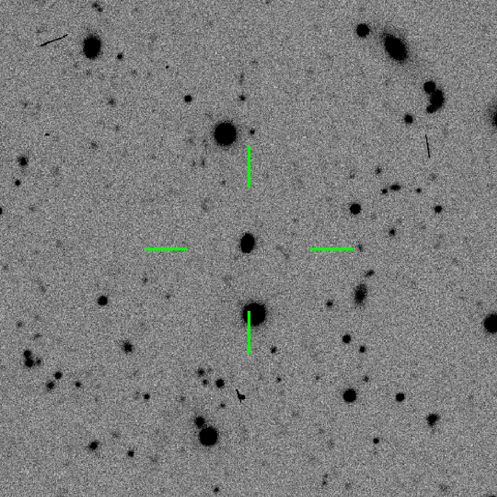
The project "workflow" is the task volunteers are asked to perform. At present, we have one concise workflow where we ask volunteers if they see activity (i.e., a tail or coma) coming from the central object, marked by a green reticle like that shown in Figure 1. The first time participants begin classifying images they are shown a tutorial we produced that demonstrates images of activity along with tips for avoiding activity lookalikes (e.g., background galaxies). During the classifying process, users may return to the tutorial at any time. Also available during the classification process is our comprehensive Field Guide, which discusses phenomena participants may encounter, such as cosmic rays.

Figure 1. This UT 2014 March 28 DECam thumbnail image of active asteroid (62412) 2000 SY178 (at center) received a score of 0.35 via our analysis system (Section 4), below the 0.473 threshold needed to qualify as an activity candidate. The faint tail seen oriented toward a position angle (PA) ∼150° north through east (roughly 7 o'clock) extends beyond the edge of the image. The image FOV is 126'' × 126'', with north up and east left, and an overlaid green reticle as shown to Active Asteroids volunteers. DECam image from Prop. ID 2014A-0479, PI: Sheppard, observer S. Sheppard.
Download figure:
Standard image High-resolution imageThe Zooniverse web structure includes several other areas important to project success. An "About" section includes pages describing (i) our research and science justification, (ii) project team members, (iii) a listing of results (e.g., publications) stemming from the project, and (iv) a frequently asked questions (FAQ) page. The "Talk" discussion boards (forums) provide a place for participants and the science team to interact and build relationships. Surprisingly, we have made discoveries that first come to light on the Talk pages, well before the subject set was fully retired (discussed below).
3.3. Subject Sets
A "subject set" is a collection of images and associated metadata (e.g., image names, object designations). We try to select a subject set size (i.e., number of images) that balances preparation overhead with turnaround time to complete subject set retirement. Smaller subject sets are fully examined by volunteers in fewer days, but each batch requires significant overhead—both effort and time—for our team to (i) prepare each batch (described below) and (ii) analyze classification data (Section 4). Conversely, large batches take longer to complete. We found a good balance to be a subject set size of ∼22,000 images, which typically needed 4 to 8 weeks for volunteers to examine (Section 8.2).
To create subject sets, we (i) assign images from HARVEST based upon selection criteria (described below), and (ii) gather images and prepare them for upload to Zooniverse by adding a green reticle (Figure 1). The ability to select objects by criteria is motivated by the need to show volunteers a variety of images, and to optimize the discovery of activity. We fully recognize that our choices impart biases, but err on the side of making the best use of volunteer efforts.
We assemble each batch as a collection of members from different dynamical classes. As of 2023 August 17, we have submitted 19 subject sets for examination, as aforementioned typically containing ∼22,000 images. The composition has changed too as we have exhausted the images of some minor-planet classes, and have de-emphasized others (e.g., near-Earth objects, NEOs) that have proven problematic for activity identification.
To improve chances for identifying activity, we prioritize selecting images of objects closer to their perihelion passage, with the assumption that activity is more likely to be present around this point in an object's orbit. We achieve this effect by sorting HARVEST images by our simple metric, "percentage to perihelion" (Chandler et al. 2018), given by

where d, q, and Q are its orbital, perihelion, and aphelion distances, respectively. This metric is more efficiently sorted than the more familiar true anomaly angle, though %T→q does not describe the direction (i.e., inbound to, or outbound from, perihelion) of the object.
By default, we only show one image of an object in a given batch, such that volunteers are examining the maximum number of individual minor planets. In cases where we have few object images remaining (e.g., Centaurs), we do increase this number. Conversely, as of 2022 October 22, we have had the option to skip objects entirely that have already been examined by volunteers at least once. This is especially useful for populations like the main-belt asteroids, where we have in our collection tens of thousands of images of unique minor planets, all essentially at perihelion.
As of 2023 August 18, we always apply further delta magnitude limits (Section 2.5). We typically require ≥2 magnitudes brighter than our computed exposure depth (i.e., Δmag ≤ −2). We consider this threshold reasonable given the project's current classification rate and projected completeness timescales (Section 8.2).
3.4. Training Set and Expert Scoring
The training system implemented by Zooniverse for Active Asteroids is designed to teach volunteers how to identify activity. We show in Section 4 that this system measurably improves activity detection ability for the vast majority of participants. The system also served to validate that the project was functioning as intended during the launch phase, and the training system continues to serve that function today.
For training purposes, we created a subject set consisting of images known to show an object displaying cometary activity at the center. To achieve this, we manually examined ∼10,000 images of known active bodies produced by the HARVEST pipeline and assigned a score to each image. The subjective scoring system, introduced in Chandler (2022), is as follows: (0) unidentifiable/missing; (1) point-source appearance; (2) vaguely fuzzy; (3) fuzzy, activity unlikely; (4) inconclusive activity indicators (coma and/or tail); (5) likely active, some ambiguity remains; (6) activity, not very ambiguous, but faint; (7) definitely active, medium-strength indicators; (8) definitely active, strong activity evidence; (9) definitely active, overwhelming activity indicators. All training images in Active Asteroids are derived from those images to which we applied a score of ≥5, our minimum threshold, for which we consider the activity to be highly likely.
Active Asteroids is configured with two training features. The first is a system that periodically shows the user a training image, at an interval that decays with user experience (determined by the number of images N they have classified), given by the probability

The second feature is a feedback system, wherein immediate feedback is given to the user about their training image classification, whether their classification was "correct" or not. While this serves as a direct training mechanism for new participants, it also serves to reinforce the abilities of experienced users and helps keep volunteers engaged in the classification process.
4. Optimizing Classification Analysis
Volunteers examine images we produce with the HARVEST pipeline (Section 2). Training images always show activity and are described in Section 3.4; images yet to be examined are referred to as "sample" images. A "classification" occurs when a volunteer clicks a "yes" or "no" button when asked if they see activity in the image. Images are randomly selected from the current subject set (Section 3.3) of images we have uploaded to Zooniverse. Each image is nominally classified by 15 unique participants before the image is "retired," with the exception of training images which are, by design, never retired. In some uncommon situations, >15 classifications occur for sample images; in those cases, we make use of the first 15 classifications.
Classification data are not static because we regularly upload new subject sets to the project. We developed the techniques described herein with a snapshot from 2022 July. At that time, 6609 unique volunteers had examined ∼170,000 images, with ∼5 million classifications in total, including training images.
4.1. Naïve Assessment Metric and Threshold
Initially, we computed, for each image i, a simple activity likelihood metric M0(i) as the ratio of "yes" classifications for the image, Yi , and the total number of classifications, i.e., the sum of yes and no, Ni , responses for that image, as

For the development of the new metrics (discussed in the subsequent section), we validated underlying premises (e.g., users become more experienced through time) as we developed the methods. The exception was this naïve metric, which served as the starting point from which we set out to improve our classification analyses.
Here, we also define the minimum "threshold," Lmin, of a metric. This serves to differentiate between images likely to show activity—and thus qualify as candidates that our team will investigate—from those that are not. For the naïve (unjustified) threshold, we chose L0 ≥ 80%. From this initial combination of metric and threshold we set out to test and improve upon our initial selection of metric and threshold.
4.2. New Metrics
Weighting based upon assessment of volunteer trends has been employed by other Citizen Science programs. For example, Gollan et al. (2012) found Citizen Scientists may on average not perform as well as professional scientists when performing the same tasks, but also that some individuals do meet or exceed that same standard.
Metric 1: Training image accuracy. This metric considers users who perform well with training data as having more expertise than those who perform poorly, thus the more expert users should be given more weight. To quantify training image performance, we measure the ratio of a user's successful training image classification, Ytraining, to their total number of training image classifications, Ttraining, as

Metric 2: log10 number of classifications. As users classify more images, they generally become more experienced, so they should be given greater weight. This metric quantifies "experience" as a log10 of the total number of classifications for a given user. We placed an upper limit of 10,000 classifications, and scaled weights to span the range of 0–1 by dividing all weights by 4 (i.e.,  ):
):

where Ttotal is the total number of images the user had examined, including training images.
Metric 3: Optimism debiasing. We found that some users identify activity much more often than would normally be expected, thus their weight needed to be lowered accordingly. Noting that the activity occurrence rate among main-belt asteroids is estimated to be roughly 1 in 10,000 (Hsieh et al. 2015; Jewitt et al. 2015; Chandler et al. 2018), we expect a low rate of "yes" classifications. Moreover, from our cursory examinations, we estimated no more than ∼1% of images should warrant being flagged as likely active. To search for bias, we first described the fraction of classifications a user, u, submits as positive by

where Yu and Nu are the total number of "yes" and "no" classifications for that user, respectively. Around 35% of users (2400) clicked "yes" over 20% of the time, indicating an optimism bias is present. Any weight based purely upon training accuracy is skewed for users selecting "yes" to most images they classify, with a potential resultant weight of unity for training accuracy while incorrectly reflecting activity detection ability. For this metric, the more frequently a volunteer sees activity, the lower their weight becomes, via

where Ysample is the number of times a user saw activity in sample images, and Tsample is the total number of sample images the user classified.
4.3. Control List and Initial Threshold
In order to test the efficacy of each metric (or combination of metrics), we maintained a "control list" of images that our team vetted and labeled as strong activity candidates. We set a threshold Lmin for each metric (i.e., L1, L2, and L3) by iteratively increasing or decreasing the threshold L in 10% increments until all control list images appeared in the final output list of candidates. We arrived at an  threshold that resulted in control list completeness for all metrics; henceforth, this served as our initial threshold when testing metrics and combinations thereof. Throughout, a secondary goal was to minimize the number of extraneous (inactive) images flagged as promising candidates, while still including those from the control list.
4.4. Incorporating Temporal Trends
Figure 2 shows combined user weights over time for 10 randomly selected users, where time here is measured only by the number of images classified. User weights typically improved, but not always (e.g., user #7 of Figure 2), indicating that one or both of the metrics not solely dependent on classification count (i.e., M1, training accuracy, or M3, optimism debiasing) must be significantly altering the weight. This finding showed (i) a need to evaluate metrics temporally, (ii) each metric may need a multiplier (weight), and (iii) we cannot assume user abilities improve over time. To capture this time-dependent weight we employed a 5th-order polynomial fit for each user's weight over time.

Figure 2. The weight for the first 1000 images for 10 unique, randomly selected users (numbered by markers 0–9) who classified between 1000 and 10,000 images. Each number represents 20 images classified, and scores are cumulative.
Download figure:
Standard image High-resolution imageWe tried combinations of metric weights, ranging from 0 to 10, for each metric (M1, M2, M3), plus 100×, 1000×, and 10,000× to test extrema. For computational efficiency, we (i) eliminated weight combinations that were integer multiples of each other that would yield identical scores, and (ii) selected only even-number weight multiples, thereby reducing the number of required compute tasks while still covering the full range of weights. We combined the weighted metrics via

where W is the combined weight for a user, W1 is the weight of M1 (training image accuracy), W2 the weight for M2 (log10 of classification count), and W3 is the weight for M3 (optimism debiasing).
We created an overall weighted likelihood score, L, computed as a ratio of the sum of an image's weighted user "yes" classifications, wY , to the sum of all the users' weights w, given by

with m the number of users who classified the image as showing activity, and k is the total number of users who classified the image.
4.5. Metric Selection and Evaluation
For each set of weight combinations we (i) calculated a score for all sample (nontraining) images using that set of weights, (ii) determined the threshold Lmin needed to include the images of our control list (Section 4.3), and (iii) recorded the number of images, If, that received a score  for that set of weights, including images not part of the control list.
We evaluated each metric independently and in combination, and compared these to the naïve metric M0. Our newly crafted method for determining which images warrant further investigation performed markedly better than the naïve method (Section 4.1). The naïve method resulted in a threshold of  for If = 2513 images (1.48% of the classified images), 795 more than our weighted method. Moreover, employing any one standalone metric alone underperformed when compared to the combined approach (If = 1718 images (1.01%), ∼1%): M1 (training accuracy) gave If = 1807 images (1.06%), M2 (number of classifications) If = 1972 images (1.16%), and M3 (optimism debiasing) returned If = 1995 images (1.17%).
We selected a final weight combination of W1 = 7, W2 = 2, and W3 = 1, with a threshold  . This combination resulted in 1718 activity candidate images for our team to examine, ∼1% of the ∼170,000 images (discussed at the beginning of this section) used for the classification analysis improvements.
We evaluated the 15 image retirement criteria (Section 3.3) by varying the number of classifications required per image prior to subject retirement. We calculated the combined weighted score for every image, considering only the first n classifications for each image, for 1 ≤ n ≤ 15. The number of extraneous images flagged for investigation declined through n = 14. While n = 14 unexpectedly performed marginally better (233 images) than n = 15, we interpret this result as indicating that 14 classifications per image represents a necessary minimum to achieve the best results for our project. We chose to keep n = 15 for the live project, in keeping with the original Zooniverse recommendation.
5. Activity Candidate Investigation
Once we have scores produced by our classification analysis system (Section 4) we next produce a list of images that match the threshold, as justified in the preceding section. We then examine each image and apply the same 0–9 scoring system described in Section 3.4. We further investigate candidates with scores ≥3, through archival and—when appropriate—follow-up telescope observations. In 2023 January, we decided to start announcing discoveries through Research Notes of the American Astronomical Society (RNAAS), especially for time-sensitive cases (e.g., the object is approaching perihelion and activity detection is useful for diagnosing the underlying mechanism). References to these publications are provided in Section 7.
5.1. Archival Investigation
Our archival investigation process typically involves first querying our internal HARVEST database for additional images of the object. This first pass enables us to quickly rule out some false-positive candidates, for example those with apparent activity that we recognize as a background source when the object is viewed in an image sequence.
For the remaining candidates, we next query external services via three pipelines we have written for the purpose, and manually query two additional sources. There are significant drawbacks to these systems as compared to HARVEST, most notably a high fraction of "junk" images that are either too faint to see the candidate, or where the candidate is not captured by a detector. Nonetheless, this in-depth search can yield images of activity that are not available through the HARVEST pipeline.
We query the following archives (see Acknowledgments for additional references) as part of the aforementioned pipelines.
CADC SSOIS. We query the CADC Solar System Object Information Search (SSOIS; Gwyn et al. 2012) for DECam, MegaPrime, Kitt Peak National Observatory instruments, Southern Astrophysical Research Telescope, SkyMapper, Las Campanas Observatory, European Space Organization instruments (e.g., Very Large Telescope Survey Telescope, VST, OMEGACam), Near-Earth Asteroid Tracking (NEAT) Ground-Based Electro-Optical Deep Space Surveillance, the Sloan Digital Sky Survey (SDSS), Subaru Suprime-Cam and Hyper Suprime-Cam, Wide-field Infrared Survey Explorer (WISE), and the Cambridge Astronomy Survey Unit Astronomical Data Centre for the Isaac Newton Telescope's Wide Field Camera data.
IRSA. With their Moving Object Search Tool (MOST), we query the NASA/CalTech Infrared Science Archive (IRSA) for Zwicky Transient Facility (ZTF) and Palomar Transient Factory data.
ZTF alert stream. We download ZTF alert stream data (Patterson et al. 2018) and keep only solar system data.
Manual queries. We manually query (i) the Keck Observatory Archive via their MOST, and (ii) the Comet Asteroid Telescopic Catalog Hub tool, which spans several instruments, including NEAT (Pravdo et al. 1999) and SkyMapper (Keller et al. 2007). After downloading the relevant data, many sources require pre- and post-processing to, for example, perform astrometry to replace an inadequate (or absent) plate solution. We perform astrometry as needed via Astrometry.net (Lang et al. 2010), which makes use of multiple source catalogs, including Gaia (Collaboration et al. 2018) and the SDSS (Ahn et al. 2012). We produce thumbnail images in FITS and PNG formats, and record sky position angle (PA) information indicating the antisolar and anti-motion vectors, as computed by JPL Horizons.
A member of the science team visually examines all of the thumbnail images produced by our follow-up pipelines and searches for activity indicators, such as tails and comae. Thus far, we have examined over two million thumbnail images as Active Asteroids follow-up and in developing the HARVEST pipeline. These data are from myriad sources and vary greatly in image quality and character (e.g., chip gaps, image orientation), and the vast majority of these data do not contain any useful information. Thus, we do not submit images from these secondary pipelines for volunteer examination.
5.2. Follow-up Observations
Objects we deem appropriate for follow-up observations are added to an internal list of candidates needing further telescope observations. Hereafter, we refer to telescopes by their name or the instrument: DECam, the Inamori-Magellan Areal Camera and Spectrograph (IMACS), the Gemini Multi-Object Spectrograph (GMOS), the Large Binocular Telescope (LBT), the Lowell Discovery Telescope (LDT), and the Vatican Advanced Technology Telescope (VATT). Table 1 lists the telescopes and facilities our team employs to carry out follow-up observations of activity candidates. We make use of ground-based facilities in both hemispheres to maximize decl. coverage. For target selection, we prioritize objects that are near perihelion (i.e., true anomaly angles of f ≥ 290° and f ≤ 70°).
Table 1. Facilities
| Instrument | Telescope | Diameter (m) | Observatory | Location | Country | Site Code |
|---|---|---|---|---|---|---|
| ARCTIC | APO | 3.5 | APO | Apache Point, New Mexico | USA | 705 |
| DECam | Blanco | 4.0 | CTIO | Cerro Tololo | Chile | 807 |
| GMOS-S | Gemini South | 8.1 | Gemini | Cerro Pachon | Chile | I11 |
| IMACS | Baade | 6.5 | Magellan | Las Campanas | Chile | 304 |
| LBCB, LBCR | LBT | 8.5 × 2 | MGIO | Mt. Graham, Arizona | USA | G83 |
| LMI, NIHTS | LDT | 4.3 | Lowell Observatory | Happy Jack, Arizona | USA | G37 |
| VATT4K | VATT | 1.8 | MGIO | Mt. Graham, Arizona | USA | 290 |
| ZTF camera | ZTF | ⋯ | ⋯ | ⋯ | ⋯ | ⋯ |
Note. Definitions: Astrophysical Research Consortium Telescope Imaging Camera (ARCTIC) Apache Point Observatory (APO), Dark Energy Camera (DECam; DePoy et al. 2008; Flaugher et al. 2015; Collaboration et al. 2016, Cerro Tololo Inter-American Observatory; CTIO), Gemini Multi-Object Spectrograph (GMOS; Hook et al. 2004; Gimeno et al. 2016), Inamori-Magellan Areal Camera and Spectrograph (IMACS; Huehnerhoff et al. 2016), Large Binocular Camera Blue (LBCB), Large Binocular Camera Red (LBCR), Large Binocular Telescope (LBT), Mount Graham International Observatory (MGIO), Large Monolithic Imager (LMI; Massey et al. 2013), Near-Infrared High-Throughput Spectrograph (NIHTS; Gustafsson et al. 2021), Lowell Discovery Telescope (LDT), Vatican Advanced Technology Telescope (VATT).
Download table as: ASCIITypeset image
6. Dynamical Classification
To gain insight into the objects we are studying, we classify them in a dynamical class, such as JFC or Centaur. A common tool employed to distinguish between different dynamical classes is the Tisserand parameter (Tisserand 1896) with respect to Jupiter, which conveys the relative influence of Jupiter on a given object's orbit, and is defined by
where e and i are the orbital eccentricity and inclination of the body, respectively, and the semimajor axis of the body and Jupiter are a and aJ, respectively.
Objects with TJ < 3 have historically been considered dynamically cometary (see, e.g., Carusi et al. 1987, 1996), whereas objects with TJ ≥ 3 have been considered dynamically asteroidal (Vaghi 1973a, 1973b). Objects with 2 < TJ < 3 are considered to be JFCs if active (Jewitt 2009), while objects with TJ < 2 are considered Damocloids (e.g., the class namesake, 5335 Damocles; McNaught et al. 1991; Asher et al. 1994) if inactive, or Halley-type comets or long-period comets, such as the retrograde, TJ = −0.395 C/2014 UN271 (Bernardinelli–Bernstein; Bernardinelli et al. 2021) if active (Jewitt 2005). Importantly, objects with TJ > 3 have orbits that do not cross the orbit of Jupiter (Levison 1996), i.e., the orbits are entirely interior or exterior to the orbit of Jupiter. It is also important to note that objects may appear to be inactive upon their initial discovery, and consequently are referred to as asteroidal even though their dynamical properties (e.g., TJ) are suggestive of a cometary body. In the interim these objects may be referred to as an asteroid on a cometary orbit (ACO; Fernández et al. 2005; Licandro et al. 2006; Kim et al. 2014), a dormant comet (Ye et al. 2016), a comet nucleus (Lamy et al. 2004), an extinct comet (Fernández et al. 2001), or a Manx comet (Meech et al. 2014).
We adopt the Jewitt (2009) definition whereby Centaurs (i) have perihelia and semimajor axes between the semimajor axes of Jupiter (aJ ≈ 5 au) and Neptune (aN ≈ 30 au), and (ii) are not in 1:1 MMR with any planet.
Membership in the quasi-Hilda family cannot be established by orbital parameters alone, although rough Tisserand parameter constraints of 2.9 ≤ TJ ≤ 3.1 have proven useful for locating candidate members (see Oldroyd 2022). To provide additional diagnostic information, we examine Jupiter corotating reference frame orbital plots (Figure 3) to establish similarities to other established quasi-Hildas, as described in Chandler et al. (2022). Hilda asteroids are in stable 3:2 interior MMR with Jupiter (Murray & Dermott 1999), but the quasi-Hildas are near, not within, this resonance. Notably, quasi-Hildas have a distinguished tri-lobal feature in the reference frame corotating with Jupiter (Figure 3(e)). We generate these plots by integrating the object of interest for 200 yr along with the Sun and the planets (excluding Mercury) using the REBOUND IAS15 N-body integrator (Rein & Liu 2012; Rein & Spiegel 2015) in python.
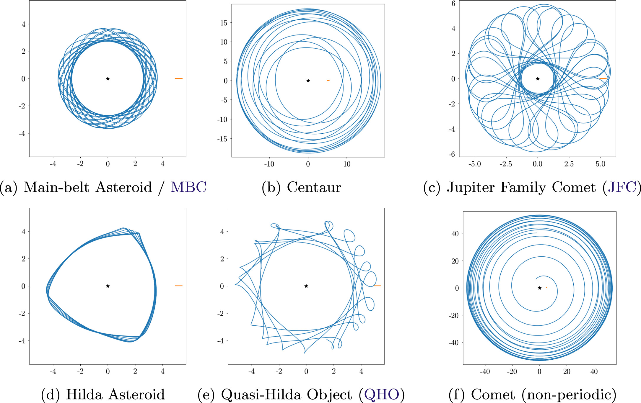
Figure 3. Example orbits of objects representing different dynamical classes, as seen in the Jupiter corotating reference frame. In all frames the Sun (star marker) is at the center, Jupiter (orange marker) is at the right, and the object is indicated by blue markers. All axes are in units of au. (a) Main-belt asteroid and MBC 133P/Elst-Pizarro. (b) Centaur (2060) Chiron. (c) Jupiter-family comet (JFC) 67P/Churyumov-Gerasimenko. (d) (153) Hilda. (e) Quasi-Hilda object (QHO) 282P. (f) Nonperiodic comet C/2020 PV6 (Pan-STARRS).
Download figure:
Standard image High-resolution image7. Results
The Active Asteroids project has prompted discoveries by our team before and after the project launch. As it is the goal of this manuscript to encapsulate all of the results stemming from our program to date, we briefly summarize all findings here and identify connections to new results introduced both in this manuscript and in the interim (Section 5). We first present our prelaunch discoveries (Section 7.1) in chronological order, and our postlaunch discoveries (Section 7.2) by dynamical class, with constituent objects sorted by provisional designation (and thus original object discovery date).
7.1. Prelaunch Discoveries
7.1.1. Active Asteroid (62412) 2000 SY178
As discussed in Section 2, we first conducted a proof of concept to demonstrate the viability of DECam data as a source of images for activity discovery (Chandler et al. 2018). We justified this determination in part by identifying one known active asteroid, (62412) 2000 SY178 (Sheppard & Trujillo 2015), after searching the 35,640 images we produced with the initial version of the HARVEST pipeline (Section 2). These images consisted of 11,703 unique minor planets, allowing us to produce a rudimentary activity occurrence rate estimate of one in ∼12,000, in rough agreement with the existing 1:10,000 estimate (Hsieh et al. 2015; Jewitt et al. 2015).
A consideration for drawing statistically robust conclusions from our project is volunteer ability to detect activity, as discussed in Section 4. For example, Active Asteroids volunteers did not flag an image of (62412) 2000 SY178 as an activity candidate as defined by our analysis system (Section 4). However, the image (Figure 1) does indeed show a faint tail and was in fact drawn from the same data in which Sheppard & Trujillo (2015) made the activity discovery. Yet we see many other instances where volunteers identified activity in known active objects that our team had difficulty spotting. With different individuals involved, both volunteer and science team, we do not find it surprising that outcomes are not entirely predictable, but we feel it is important to emphasize the point here. These considerations reinforce the need for many volunteers to examine a given image.
7.1.2. Active Asteroid (6478) Gault
In 2019 January, asteroid (6478) Gault (Figure 4(a); Prop. ID 2012B-0001, PI: Frieman, observers SK, DT, NFM) was reported to be displaying activity (Hui et al. 2019; Jewitt et al. 2019; Marsset et al. 2019; Moreno et al. 2019; Smith et al. 2019; Ye et al. 2019; Devogèle et al. 2021). For the first time, our team made use of the HARVEST pipeline, which was not yet complete, to identify images of Gault in DECam data. In Chandler et al. (2019), we reported our subsequent discovery that Gault had been active during multiple prior epochs. We found Gault's activity was not correlated with perihelion passage, and we postulated that Gault is recurrently active due to rotational spin-up, supported by Kleyna et al. (2019) findings of YORP-induced effects on Gault. Our findings stemmed from tools we created to help us understand potential observational biases and correlation effects with perihelion passage and activity outbursts.

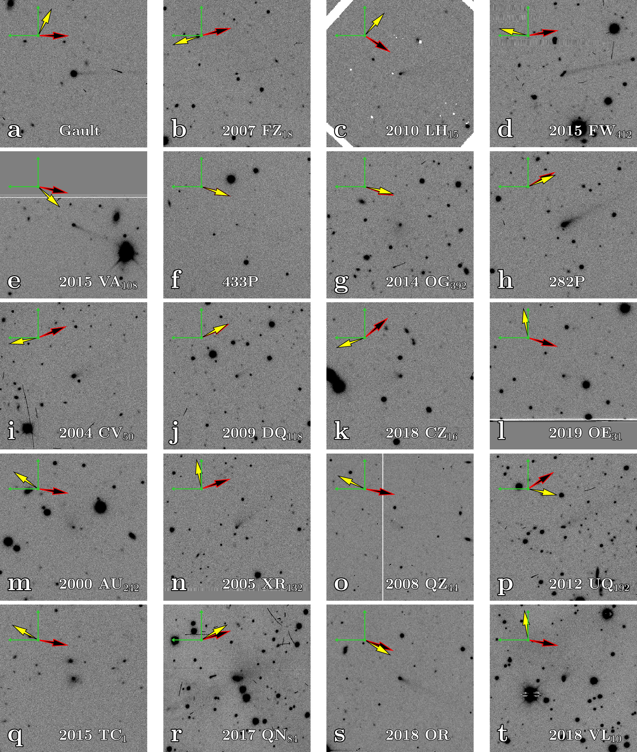
Figure 4. Minor planets with activity discoveries resulting from the Active Asteroids project. (a)–(f) are active asteroids and MBC candidates; (g) is an active Centaur; (h)–(l) are active QHAs; (m)–(t) are JFCs. In all panels the object is at center, north is up and east is left, and the FOV is 126'' × 126''. The antisolar (yellow filled arrow) and anti-motion (black arrow with red border) directions as projected on sky are shown in the top-left corner of each image.
Download figure:
Standard image High-resolution imageEven with this strategy in place, both observability (the number of hours an object is above the horizon as observed from a given observatory) and perihelion passage must be coincident to maximize the chances an object will be shown to volunteers. For example, only the 2016 perihelion passage coincided with a peak in observability. At other times (e.g., 2013, 2019) Gault was highly observable, but it was not near perihelion, or Gault was minimally observable (or not observable) at perihelion, as was the case in 2012.
7.1.3. Active Centaur C/2014 OG392 (Pan-STARRS)
Our team discovered activity emanating from Centaur 2014 OG392 (Figure 4(g); Prop. ID 2019A-0337, PI: Trilling, observer C. Trujillo), now designated C/2014 OG392 (Pan-STARRS) following our discovery, while testing our project workflow in preparation for the Active Asteroids program. As part of this testing we treated the object as if it had been discovered by volunteers, first carrying out an archival investigation, then follow-up telescope observations, as described in Section 5. We successfully confirmed the presence of activity during our own observations with DECam (UT 2019 August 30, 250 s VR band; Prop. ID 2019A-0337, PI: Trilling, observer C. Trujillo) on UT 2019 August 30 (Chandler et al. 2020). Given the elapsed time between the archival activity and new observations, it is likely the object had been active for years. Additional observations we obtained with the 4.3 m LDT enabled us to classify C/2014 OG392 as a red centaur (see review by Peixinho et al. 2020), to estimate a diameter of 20 km, and carry out mass-loss estimates. We also introduced a novel technique to estimate the species likely responsible for sublimation at the experienced orbital distances, in this case carbon dioxide and/or ammonia.
Since project launch we have submitted all thumbnail images available of Centaurs for classification. Project volunteers did identify C/2014 OG392 as active, including the original archival images that prompted our publication, as well as the new observations we conducted. Moreover, volunteers identified activity in images of other known active Centaurs. However, while we are actively investigating several leads stemming from Active Asteroids, C/2014 OG392 remains the only active Centaur discovery by our program thus far.
7.1.4. Main-belt Comet 433P
Just prior to project launch, (248370) 2005 QN173, subsequently designated 433P, was discovered to be active (Fitzsimmons et al. 2021). In addition to the HARVEST pipeline, we also debuted our secondary pipelines developed for archival investigation (Section 5.1). We successfully identified 81 images of the object, spanning 31 observations, in which we could confidently identify 433P. Of these, we found a single image (Figure 4(f)), dated UT 2016 July 22 (Prop. ID 2016A-0190, PI: Dey, observers D. Lang, A. Walker), that showed 433P unambiguously active with a long, thin tail oriented toward the coincident antisolar and anti-motion vectors as projected on sky (Chandler et al. 2021). Our discovery of a previous activity epoch that occurred near perihelion, along with 433P's probably C-type spectral class (Hsieh et al. 2021), allowed us to classify the object as a MBC. At the time, just ∼15 of these objects were known.
We introduced wedge photometry as an activity detection and measurement tool in Chandler et al. (2021). This tool, which shares similarities to one by Sonnett et al. (2011), measures flux in annular regions around a target, using different angular wedge sizes, to identify the presence of a tail and to measure its angle for comparison with ephemeris computed antisolar and anti-motion projected vectors. As with Ferellec et al. (2022), who developed a similar tool around the same time, we found background sources to significantly impede the practicality of this approach. In the future, especially for surveys with high-quality templates—as should be the case for the Legacy Survey of Space and Time (LSST)—the tool may be of practical use to filter out false positives and thus improve the overall quality of images we provide volunteers for classification.
7.2. Postlaunch Discoveries
For the remainder of this section, we discuss 16 objects, all classified as active by Active Asteroids volunteers and brought to our team's attention as a result. A representative thumbnail showing activity for each object is provided in Figure 4. We classify each object into a dynamical class, and in the process refer to (i) object-specific properties (e.g., inclination, perihelion distance), and (ii) the gallery of Jupiter corotating reference frame plots (Figure 5). Table 3 provides a unified collection of data pertaining to the observed activity, most notably the date ranges of activity along with corresponding heliocentric distances rH and true anomaly angles f.
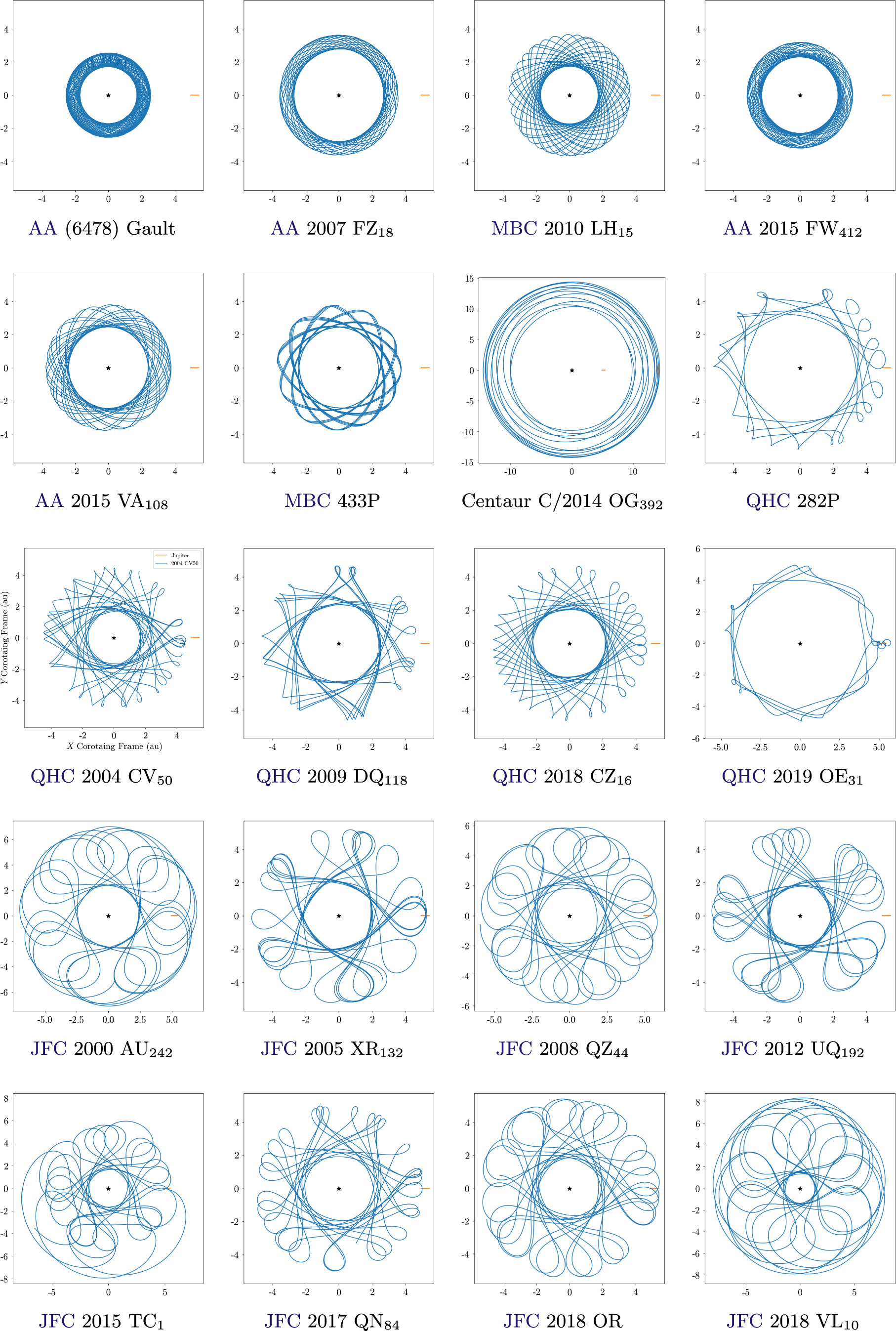
Figure 5. Jupiter corotating frame plots for the objects presented in this work. In all panels, the Sun (star marker) is at the center, with Jupiter and the minor planet indicated by orange and blue markers, respectively. All axes are in units of au. Acronyms: active asteroid (AA), Jupiter-family comet (JFC), main-belt comet (MBC), and quasi-Hilda comet (QHC).
Download figure:
Standard image High-resolution image
With the exception of 282P/(323137) 2003 BM80, all objects are referred to by their primary provisional designation, with full and alternate designations for each object listed in corresponding subsections. In the tables and subsections provided, we generally group objects by dynamical class first, then sort objects by provisional designation within each dynamical class.
7.2.1. Active Asteroids
The Active Asteroids program has thus far led us to discover four new active asteroids: 2007 FZ18, 2010 LH15 (seen to be active at two apparitions), 2015 FW412, and 2015 VA108. They have TJ values ranging from TJ = 3.160 to TJ = 3.351, placing them all firmly outside of the JFC or quasi-Hilda regimes. As indicated in Table 3, all activity took place near perihelion passages, with the earliest activity at a true anomaly angle f = 320°, and the latest f = 33°. For all active asteroids we identified, this behavior is consistent with sublimation-driven activity, and thus these objects are all MBC candidates. The recurrent activity we found for 2010 LH15 is additional evidence supporting sublimation-driven activity as the underlying mechanism, thus it is likely an MBC.
(588045) 2007 FZ18. A single thumbnail image of 2007 FZ18 (Figure 4(b); 60 s DECam VR-band image from UT 2018 February 15; Prop. ID 2014B-0404, PI: Schlegel, observer S. G. A. Gontcho) was classified by Active Asteroids volunteers as showing evidence of activity (Chandler et al. 2023a). A long, thin tail is visible in the anti-motion direction, with a PA ∼300° east of north (roughly 2 o'clock), and a shorter, fainter tail seen extending toward the antisolar direction (PA ∼ 300° east of north, about 8 o'clock). At the time, 2007 FZ18 was outbound from its perihelion passage with a true anomaly angle of f = 4.8°, at a heliocentric distance rH = 2.80 au. 2007 FZ18 (a = 3.18 au, e = 0.12, i = 1.1°, q = 2.78 au, Q = 3.57 au), with TJ = 3.188, is a main-belt asteroid. The activity occurred when 2007 FZ18 was at rH = 2.80 au, on UT 2018 February 15, outbound from perihelion at f = 4.8°, consistent with sublimation-driven activity. Thus, (588045) 2007 FZ18 is a candidate MBC.
2010 LH15 . We found 2010 LH15, also designated 2010 TJ175, was active spanning UT 2010 September 27, heliocentric distance rH = 1.79 au and true anomaly angle f = 21.5°, to UT 2010 October 7, rH = 1.80 au and f = 32.6° (Chandler et al. 2023b). An image from this first activity epoch is provided in Figure 4(c) (UT 2010 October 6 40 s r-band Pan-STARRS 1 image). We identified a second epoch of activity in images (e.g., UT 2019 September 30 90 s DECam exposure; Prop. ID 2019B-1014, PI: Olivares, observers F. Olivares, I. Sanchez) spanning from UT 2019 August 10 (rH = 1.78 au, f = 346°) through 2019 October 31 (rH = 1.81 au, f = 25°). 2010 LH15 (a = 2.74 au, e = 0.36, i = 10.9°, q = 1.77 au, Q = 3.72 au), with TJ = 3.230, is a main-belt asteroid, and its recurrent activity near perihelion indicates the object is an MBC.
2015 FW412. We identified 2015 FW412 (Figure 4(d); UT 2015 April 13; Prop. ID 2015A-0351, PI: Sheppard, observers S. Sheppard, C. Trujillo) activity in DECam images from when 2015 FW412 was at rH = 2.40 au and inbound to perihelion at f = 320°. We found ∼20 images showing the object with a clear tail oriented in the anti-motion direction, roughly toward 3 o'clock, or PA ∼270° east of north (Chandler et al. 2023c). Additional images of activity include DECam on UT 2015 April 18 (Prop. ID 2013B-0536; PI Allen, observers L. Allen, D. James). 2015 FW412 (a = 2.76 au, e = 0.16, i = 13.7°, q = 2.32 au, Q = 3.21 au) has TJ = 3.280 and is thus a main-belt asteroid. Its activity near perihelion is consistent with sublimation, thus this object is an MBC candidate.
2015 VA108. Volunteers classified an image of 2015 VA108 (Figure 4(d); UT 2015 October 11 DECam; Prop. ID 2014B-0404, PIs: Schlegel and Dey, observers D. James, A. Dey, A. Patej) as showing activity, and our investigation revealed one additional image, acquired during the same UT 2015 October 11 observing night (Chandler et al. 2023d). In both images a prominent tail is seen oriented toward the antisolar and anti-motion directions, roughly 4 o'clock (PA ∼ 240°). At the time, 2015 VA108 was outbound from perihelion at f = 15.68° and rH = 2.44 au. 2015 VA108 (a = 3.13 au, e = 0.22, i = 8.5°, q = 2.45 au, Q = 3.81 au) has TJ = 3.160 and thus is a main-belt asteroid. Its activity near perihelion is suggestive of sublimation, thus this body is an MBC candidate.
7.2.2. Quasi-Hilda Objects
Active Asteroids volunteers identified activity associated with five minor planets, spanning eight activity epochs, which our dynamical classification scheme (Section 6) identified as a QHA: 282P, 2004 CV50, 2009 DQ118, 2018 CZ16, and 2019 OE31. All activity we found took place relatively near perihelion passage, with true anomaly angles ranging from f = 322° to f = 37°, with the most distant activity taking place at 3.92 au (Table 3).
282P/(323137). The minor planet 2003 BM80 (Figure 4(h); Prop. ID 2019A-0305, PI: Drlica-Wagner, observer T. Li), was known to be active (Bolin et al. 2013). Active Asteroids volunteers identified activity from two different epochs, with the more recent activity epoch being a new finding (Chandler et al. 2022) from our follow-up observing campaign with the GMOS-S instrument on the 8.1 m Gemini South telescope (Prop. ID GS-2022A-DD-103, PI: Chandler), with preparatory observing at the VATT and LDT. Our modeling efforts showed 282P (a = 4.24 au, e = 0.19, i = 5.8°, q = 3.44 au, Q = 5.03 au) has a short dynamical lifetime of roughly ±300 yr and, at present, is a QHO.
2004 CV50. Volunteers of Active Asteroids classified an image of 2004 CV50 (Figure 4(h); DECam; Prop. ID 2020A-0399; PI: Zenteno, observer A. Diaz) as active (Chandler et al. 2023e). Our subsequent archival image search (Section 5.1) revealed two additional images of activity for a total of three images spanning two different dates. For these two dates (UT 2020 February 15 and UT 2020 March 14), 2004 CV50 was inbound at a heliocentric distance of rH = 1.68 au (f = 343°) and rH = 1.66 au (f = 359°), respectively. Our dynamical modeling (Section 6) indicates 2004 CV50 (TJ = 3.061, a = 3.10 au, e = 0.44, i = 1.4°, q = 1.73 au, Q = 4.48 au) is an active QHO rather than an active asteroid, despite the object's TJ > 3.
2004 CV50 does not cross Jupiter's orbit, though it has had, and will have, close encounters with Jupiter.
2009 DQ118. We found >20 images of activity of 2009 DQ118 (Figure 4(j); Prop. ID 2016A-0189, PI: Rest, observers A. Rest, DJJ) with activity from this epoch, spanning two consecutive days, from UT 2016 March 8 to UT 2016 March 9, when 2009 DQ118 was at a rH = 2.55 au and f = 322° (Oldroyd et al. 2023a). Our follow-up observations with the Astrophysical Research Consortium instrument on the Apache Point Observatory (APO) 3.5 m telescope (Sunspot, NM, USA) and the Inamori-Magellan Areal Camera and Spectrograph(IMACS) instrument on the 6.5 m Baade Telescope (Las Campanas Observatory, Chile) revealed 2009 DQ118 was active again, indicating that sublimation is the most likely mechanism responsible for the observed activity (Oldroyd et al. 2023b). Our dynamical modeling (Section 6) indicated 2009 DQ118 (TJ = 3.004, a = 3.58 au, e = 0.32, i = 9.4°, q = 2.43 au, Q = 4.72 au) is an active QHO.
2018 CZ16. We found a total of four DECam images of 2018 CZ16 (Figure 4(k); UT 2018 May 15, 17 and 18, DECam; Prop. ID 2014B-0404, PI: Schlegel, observers E. Savary, A. Prakash) displaying activity (Trujillo et al. 2023). These images span UT 2018 May 15 to UT 2018 May 18, when 2018 CZ16 was inbound at heliocentric distances of rH = 2.295 au and rH = 2.292 au, respectively, and true anomaly angles of f = 344° to f = 345°. We classify 2018 CZ16 (TJ = 2.995, a = 3.45 au, e = 0.34, i = 13.7°, q = 2.27 au, Q = 4.63 au) as an active QHO via our dynamical classification system (Section 6).
2019 OE31. Volunteers identified activity in a DECam image of 2019 OE31 (Figure 4(l); UT 2019 August 9; Prop. ID 2019A-0305, PI: Drlica-Wagner, observers T. Li, K. Tavangar). We later learned activity had been independently identified by S. Deen on 2021 May 15 and reported on Seichi Yoshida's Comet Pages. 23 We identified two additional images showing possible activity from UT 2019 August 9 (heliocentric distance rH = 3.92 au, true anomaly f = 3°) and UT 2019 September 30 (rH = 3.93 au, f = 10°). Notably, 2019 OE31 has very close encounters with Jupiter (e.g., 0.017 au on UT 2013 October 1; retrieved UT 2023 September 25 from JPL) that significantly altered its orbit, making archival investigation difficult for data prior to 2013. By our dynamical classification system (Section 6), 2019 OE31 (TJ = 3.006, a = 4.37 au, e = 0.10, i = 5.2°, q = 3.93 au, Q = 4.82 au) is an active QHO. We discuss the Centaur origin of 2019 OE31 in Oldroyd et. al (2023c).
7.2.3. Jupiter-family Comets
Our program identified seven new active objects with Tisserand parameters with respect to Jupiter 2 < TJ < 3 (typically classified as JFCs; see Section 6): 2000 AU242, 2005 XR132, 2012 UQ192, 2015 TC1, 2017 QN84, 2018 OR, and 2018 VL10.
2000 AU242. During project preparations we identified a single DECam image of (275618) 2000 AU242 (Figure 4(m); Prop. ID 2014B-0404, PI: Schlegel, observers A. Dey, S. Alam) that showed conspicuous activity indicators (Chandler 2022). (275618) 2000 AU242 was at rH = 5.91 au, inbound from aphelion (f = 218.91°). Project volunteers identified the same image as showing activity. Our archival investigation did not uncover any additional images of unambiguous activity, and our own observing campaign with the 4.3 m LDT on UT 2021 January 10 (PI: Chandler, observers C. Chandler, C. Trujillo), when (275618) 2000 AU242 was at rH = 2.90 au, near perihelion (f = 302.5°), and UT 2020 February 3 (PI: Gustafsson, observers A. Gustafsson, C. Chandler) when (275618) 2000 AU242 was at rH = 4.35 au and f = 251.1°, showed (275618) 2000 AU242 was most likely quiescent. With TJ = 2.738, (275618) 2000 AU242 (a = 4.80 au, e = 0.49, i = 9.5°, q = 2.46 au, Q = 7.14 au) is a member of the JFCs.
2005 XR132. Active Asteroids volunteers classified a DECam image of 2005 XR132 (Figure 4(m); UT 2021 March 26; Prop. ID 2021A-0149, PI: Zenteno, observer A. Zenteno) as showing activity, and our archival investigation revealed additional activity images from the ZTF (Chandler et al. 2023f). 2005 XR132 had previously been reported as active (Cheng et al. 2021a, 2021b) in images from another observatory, but 2005 XR132 had not yet received a comet destination. We identified hints of activity as early as UT 2021 January 3, though activity is more definitively identifiable beginning UT 2021 February 8 (rH = 2.21 au and f = 27.1°). The last image of clear activity, from ZTF, is from UT 2021 March 21 (rH = 2.31 au and f = 40.9°). We classify 2005 XR132 (TJ = 2.869, a = 3.76 au, e = 0.43, i = 14.5°, q = 2.14 au, Q = 5.38 au) as a JFC.
2008 QZ44. We identified activity in 2008 QZ44 (Figure 4(o); UT 2008 November 20 Canada–France–Hawaii Telescope MegaPrime; PI: Hoekstra, observers the "QSO Team") via two independent means (Chandler et al. 2023g). A member of our team discovered images of 2008 QZ44 as part of a separate investigation, and volunteers from the Active Asteroids project flagged two images of 2008 QZ44 as showing activity. The nine MegaPrime images, all from UT 2008 November 20 (rH = 2.43 au and f = 29°), clearly show a tail in the antisolar direction. The second activity epoch (UT 2017 November 12–13, rH = 2.90 au, f = 68°; Prop. ID 2014B-0404, PI: Schlegel, observers C. Stillman, J. Moustakas, M. Poemba) is visible in DECam images as a tail oriented between the antisolar and anti-motion angles. We classify 2008 QZ44 (TJ = 2.821, a = 4.19 au, e = 0.44, i = 11.4°, q = 2.35 au, Q = 6.04 au) as a JFC.
2012 UQ192. Volunteers flagged (551023) 2012 UQ192 (Figure 4(p); UT 2014 April 30; Prop. ID 2014A-0283, PI: Trilling, observers D. Trilling, L. Allen, J. Rajagopal, T. Axelrod), alternate designation 2019 SN40, as showing activity (DeSpain et al. 2023). Our follow-up archival investigation revealed a total of four images from the same orbit that showed an unambiguous tail oriented toward the anti-motion direction, PA ∼300° east of north (roughly the 2 o'clock position). At the time, (551023) 2012 UQ192 was outbound from perihelion. Activity is evident in DECam images from UT 2014 April 30 (rH = 2.99 au, f = 96.5°), UT 2014 May 5 (rH = 3.02 au, f = 97.5°), and in >20 ZTF images between UT 2020 November 12 (rH = 2.08 au, f = 40°) and UT 2021 May 5 (rH = 2.84 au, f = 90°). With recurrent activity near perihelion, the activity is most likely caused by sublimation. We classify (551023) 2012 UQ192 (TJ = 2.824, a = 3.69 au, e = 0.48, i = 16.6°, q = 1.82 au, Q = 5.47 au) as a JFC.
2015 TC1. We reported 2015 TC1 (Figure 4(q); UT 2015 December 19) activity in Chandler (2022); however, Active Asteroids volunteers subsequently identified additional images of activity. All images are from DECam and part of Prop. ID 2012B-0001 (PI: Frieman, observers S. S. Tie, B. Nord, D. Tucker, T. Abbott, C. Furlanetto, J. Allyn Smith, E. Balbinot, D. Gerdes, S. Jouvel). Images of activity span from UT 2015 October 7 (rH = 2.00 au, f = 28°) to UT 2016 January 1 (rH = 2.29 au, f = 59°). We classify 2015 TC1 (TJ = 2.789, a = 3.77 au, e = 0.49, i = 17.8°, q = 1.91 au, Q = 5.64 au) as a JFC.
2017 QN84. 2017 QN84 activity (Figure 4(r); UT 2017 December 23; Prop. ID 2017B-0307, PI: Sheppard) was identified by Active Asteroids participants and initially reported on project forums. While we only identified a single image of 2017 QN84 with activity, we produced a comparison image that clearly demonstrates there were no background sources that could be mistaken as activity (Chandler 2022). Moreover, the activity extends from 2017 QN84 toward the coincident antisolar and anti-motion directions (as projected on sky), approximately 2 o'clock (PA ∼300° east of north), suggesting a physical phenomenon rather than an image artifact. On the date we see the activity, 2017 QN84 was outbound at rH = 2.62 au and f = 38°. We classify 2017 QN84 (TJ = 2.944, a = 3.77 au, e = 0.34, i = 12.1°, q = 2.48 au, Q = 5.06 au) as a JFC.
2018 OR. We identified images of 2018 OR (Figure 4(s)) showing activity (Farrell et al. 2024) beginning UT 2018 September 5 (rH = 1.64 au, f = 8.2°) and as late as UT 2018 September 18 (rH = 1.66 au, f = 15.6°). The images date from UT 2018 September 5 (MegaPrime; Prop. ID 18BH09, PI: Wainscoat), UT 2018 September 6, and UT 2018 September 18 (DECam; Prop. ID 2014B-0404, PI: Schlegel, observers A. Slepian, D. Schlegel), and ZTF on UT 2018 September 17. Notably, 2018 OR (TJ = 2.861, a = 3.53 au, e = 0.54, i = 2.1°, q = 1.64 au, Q = 5.43 au) crosses the orbit of Mars and is nominally labeled an "outer grazer" as 2018 OR has a perihelion distance interior to Mars' aphelion distance, yet exterior to Mars' semimajor axis. We classify 2018 OR as a member of the JFCs.
2018 VL10. The DECam images of 2018 VL10 (Figure 4(t); UT 2018 December 31; Prop. ID 2018B-0122, PI: Rest, observers A. Zenteno, A. Rest) that we identified as having activity (Chandler et al. 2023i) range from UT 2018 December 31 (rH = 1.42 au, f = 0.0°) to UT 2019 February 01 (rH = 1.47 au, f = 23°). 2018 VL10 (a = 4.59 au, e = 0.69, i = 18.5°, q = 1.42 au, Q = 7.76 au) qualifies as a Mars-crosser of the "outer grazer" subtype (see 2018 OR above for definition). With a TJ = 2.420, we classify 2018 VL10 as a JFC. Notably, 2018 VL10 came within 0.479 au of Earth on UT 2019 January 9, and will approach closer yet (0.429 au) on UT 2087 January 11. However, with q = 1.42 au, 2018 VL10 does not qualify as an NEO by the Center for Near Earth Object Studies definition, which places an outer bound of qNEO ≤ 1.3 au.
7.3. Classification Metrics
We describe here a brief preliminary analysis of the Active Asteroids classifications and results. We caution that (i) the inferences herein have not been debiased in any way, and we impart significant biases in our subject selection process (e.g., we sort objects submitted for classification by distance from perihelion; see Section 3.3); (ii) that the classifications are incomplete (e.g., ∼241,000 of ∼1.1 million main-belt asteroids have been examined by the project thus far); (iii) our investigation into newfound activity epochs is ongoing; and (iv) some dynamical classifications require dynamical simulations (Section 5), and thus may have been incorrectly labeled in the past. While we primarily make use of the object class returned by the Quaero service (Berthier et al. 2006), some classes contain objects with ambiguous membership, e.g., JFCs that also qualify as NEOs.
Table 2 shows metrics by object class, with analyses considering subjects (images) and unique objects. Overall, Active Asteroids volunteers classified 1.3% of the images as showing activity, with our team concurring 33.3% of the time (i.e., 0.04% of all images examined). We investigated these candidates (Section 5) except for training images (Section 3.4), which are included in Table 2 to indicate, for example, volunteer expertise (Section 4).
Table 2. Preliminary Metrics for Subjects and Objects Examined
| Class | Subjects Examined | CitSciyes | Objects Examined | CitSciyes | Activity Discoveries |
|---|---|---|---|---|---|
| Asteroid | 300,526 | 2707 | 240,989 | 25 | 6 a |
| Comet | 1605 | 1002 | 399 | 399 | 0 |
| JFC+ACO | 13,394 | 590 | 3300 | 212 | 8 b |
| Centaur | 2092 | 49 | 193 | 11 | 1 c |
| Other | 113,115 | 1272 | 37, 097 | 36 | 5 d |
| Total | 430,732 | 5620 | 281,978 | 683 | 20 |
Notes. "Subjects Examined" indicates the number of thumbnail images examined by project volunteers. "Objects Examined" are the number of unique minor planets examined by project volunteers. "CitSciyes" indicates the number of images or objects flagged as active by volunteers. "Activity Discoveries" indicates activity discoveries by our campaign before and after project launch, including activity on objects not known to be active and newfound activity apparitions. Abbreviated is CitSci (Citizen Science project volunteers). Asteroids have TJ > 3. Comets indicate long-period and hyperbolic comets, TJ < 2. JFC and ACO have 2 < TJ < 3. Centaurs have a and q between Jupiter and Neptune's aphelia distances. "Other" includes Hilda asteroids, Hungaria asteroids, interstellar objects, Mars-crossing asteroids, NEOs, TNOs, Trojan asteroids, and QHOs.
a Section 7.2.1: Gault (Chandler et al. 2019), 2007 FZ18 (Chandler et al. 2023a), 2010 LH15 (Chandler et al. 2023b), 2015 FW412 (Chandler et al. 2023c), 2015 VA108 (Chandler et al. 2023d), 433P (Chandler et al. 2021; Hsieh et al. 2021). b Section 7.2.3: 2000 AU242 (Chandler 2022), 2005 XR132 (Cheng et al. 2021b; Chandler et al. 2023f), 2008 QZ44 (Chandler et al. 2023g), 2012 UQ192 (DeSpain et al. 2023), 2015 TC1 (Chandler 2022), 2017 QN84 (Chandler 2022), 2018 OR (Farrell et al. 2024), 2018 VL10 (Chandler et al. 2023i). c Section 7.1.3: C/2014 OG392 (Chandler et al. 2020). d Section 7.2.2: 282P (Chandler et al. 2022), 2004 CV50 (Chandler et al. 2023e), 2009 DQ118 (Oldroyd et al. 2023a, 2023b), 2018 CZ16 (Trujillo et al. 2023), 2019 OE31 (Oldroyd et al. 2023c).Download table as: ASCIITypeset image
Despite the disclaimers mentioned above, especially regarding biases and classification incompleteness, we can still make some rough inferences. Of the 240,989 unique asteroids examined by volunteers, they labeled 25 (0.010%) as showing activity, consistent with prior activity occurrence rate estimates, roughly 1 in 10,000 (Hsieh et al. 2015; Jewitt et al. 2015; Chandler et al. 2018), or 0.01%. Active Asteroids volunteers examined 193 Centaurs, of which 11 (5.7%) qualified as activity candidates by our enhanced classification analysis (Section 4).
To assess the Centaur activity occurrence rate in the context of the broader Centaur population, we first needed a list of Centaurs from which we shall make our comparisons. We also must define a Centaur as these objects are described by multiple definitions in the literature. Derived from Jewitt (2009), we define a Centaur as an object (i) with a semimajor axis a and perihelion distance q between the aphelion distances of Jupiter and Neptune (i.e., QJ < a < QN, QJ < q < QN), and (ii) not in 1:1 MMR with a giant planet. This latter requirement excludes the 24 Neptune Trojans and two Uranus Trojans known as of UT 2023 December 9, and the a and q constraints exclude objects that cross the orbit of Jupiter.
We queried the MPC list of Centaurs and scattered-disk objects 24 and the JPL Small Body Database via their query tool 25 for objects that match our a and q requirements. The results largely overlapped, noting that (i) the MPC did not include objects with comet designations in their list, and (ii) in two cases (2010 HM23 and 2015 FZ397), orbital element disagreement between the two services (e.g., 2010 HM23 a = 32.35 au via JPL and a = 27.90 via the MPC) caused an object to appear on one list but not the other. In both cases, we included the objects on our final list. Subsequently, we removed the known Trojans.
Of the 346 Centaurs on our list, 31 are active Centaurs, indicating an activity occurrence rate among the Centaurs of about 9%. This figure is in agreement with Peixinho et al. (2020), and lower than the 13% rate of Jewitt (2009) that was measured when only 92 Centaurs were known (of which 12 were active). Because Active Asteroids volunteers only examined images of about half of the known Centaurs, it is unsurprising that the 5.7% identification rate differs from our 9% rate.
Similarly, we consider the ratio of JFCs to ACOs, where the former have shown activity and the latter have not (Licandro et al. 2006, 2016). We queried the JPL Small Body Database for objects with Tisserand parameters with respect to Jupiter 2 < TJ < 3, the canonical range for JFCs, and excluded the Jupiter Trojans as well as all objects from our Centaur list. We note that we only counted one object per parent designation (i.e., we excluded fragments except for the primary designation). We flagged each object on our list as either active or inactive, based on their cometary designation or lack thereof, and we also flagged the 13 qualifying objects included in this work as active, plus another established active object, 2008 GO98 (García-Migani & Gil-Hutton 2018). Of the 14,407 minor planets on our ACO+JFC list, 668 have been observed to be active. Thus, we find the apparent occurrence rate (i.e., observed fraction) of active objects in the ACO+JFC population to be 4.6%. We reiterate our query did not restrict our population selection by any physical property (e.g., albedo or color; Licandro et al. 2016) other than observed activity, and we did not limit our ACOs or JFCs populations using the Tancredi (2014) method.
The other classes cannot be meaningfully evaluated at this time due to, for example, currently unresolved ambiguities in overlapping class definitions (e.g., JFC, QHC).
8. Discussion
8.1. Volunteer/Expert Agreement
We carried out analyses to better understand performance when classifying data. Here, we discuss the total number of submitted thumbnail images, as well as metrics from select dynamical classes of relevance to this discussion. At the time of these analyses, there were 406,082 sample (i.e., nontraining) images in the Active Asteroids project on Zooniverse. Of these, 4171 (1.03%) of the images qualified as candidates by our analysis system (Section 4). Our team flagged 526 (12.6%) of these candidates as warranting additional investigation, which we define as reaching a threshold of ≥4 based on our activity likelihood score (Section 3.4).
If we do not limit our assessment to candidates flagged by volunteers, we found an additional 138 thumbnail images that our team had previously flagged as candidates that the project had not; these images are members of dynamical classes that we examined extensively during project preparations.
The lowest fraction of objects classified as candidates by volunteers were the main-belt asteroids. Of the 300,526 images of main-belt asteroids submitted for classification (Table 7.3), 2707 (0.9%) qualified as candidates based on analysis of volunteer classifications. Of these, our team flagged 258 (9.5%) as warranting follow-up. Conversely, the highest fractions occurred with the comets. Of the 1150 sample (nontraining) images of known comets, 300 (26.1%) were flagged as candidates, and 267 (89.0%) of these our team also classified as warranting follow-up.
8.2. Thumbnail Classification Rate and Completeness
As of 2023 July 3—the date of our last Zooniverse data export—volunteers averaged 12,770 ± 10,750 classifications day–1, with a maximum rate of 129,338 classifications day–1 taking place on the project launch date, 2021 August 31. These figures include both training and sample images, and exclude dates with <1000 classifications, which typically occur when no new sample data are available on the project for volunteers to classify. Of the 6,543,368 classifications in this data export, 353,058 (5.4%) were training images. Taking this training fraction into account, the mean retirement rate (nominally 15 classifications per image; see Section 3) is 805 ± 678 sample images day–1, and our nominal peak rate covers ∼8000 sample images day–1.
Some of the variation we observe in the classification rate is due to external factors, such as media attention and publications of our findings. Internal factors are driven by when we email newsletters to participants, and lulls between subject sets are due to pauses instilled while we examine previous results and prepare a new batch. The cause of the remaining variation is unknown, though we have speculated that seasonal societal effects, such as vacation times, for example, may be partially responsible. Nevertheless, with nearly 2 yr of data to draw upon, we will consider the average and peak rates mentioned above for the remainder of this discussion.
It is worth mentioning here that we typically consider three modes of optimizing results through our Citizen Science project. All three modes can either increase the number of images examined or reduce the time it takes to complete the examination of an entire subject set. (i) Additional participation by existing volunteers, or an increased number of participants. (ii) Optimized analysis of classification data that is capable of reducing the time to retirement for at least a portion of subjects in a subject set. (iii) Reducing the amount of data needing classification, through either (a) more advanced automated vetting, or (b) measured decisions to exclude certain data. The discussion that follows focuses on decisions to reduce the volume of data. Yet we continue to work toward improving all three areas, especially techniques involving applications of artificial intelligence (AI). However, those areas are still under development and outside the scope of this manuscript.
8.2.1. Current DECam Dataset
Time to complete existing thumbnails. HARVEST has produced roughly 18 million vetted thumbnail images (Section 2). At the peak rate (8000 images day−1) this works out to 2250 days, or about 6 yr until our program has classified all of the DECam-derived images, though this assumes the data set is static (it is not; see below). At the mean rate, however, the completion time would be 22,360 days, or roughly 60 yr.
Staying current. So far, Active Asteroids has exclusively shown volunteers DECam images, from instrument first light (2012 September) to present. The archive continues to grow, and HARVEST runs daily. We estimate the occurrence of minor-planet images to be that of our average number of vetted thumbnail images produced per day, ∼5000. At our current average daily retirement rate of 805 images day−1, there is a significant deficit (i.e., we will not catch up at this rate). The peak rate (8000 images day−1) would be sufficient to stay current but would result in significant delays in processing the remainder of the existing thumbnails (see below).
Time to completion while staying current. As mentioned above, we are not presently able to examine 100% of the thumbnails produced daily by the HARVEST pipeline. The peak rate would leave just 9 hr (0.375 days) daily for classifying the remaining 18 million images. In this case, it would take roughly 16 yr to get caught up while also staying current with newly available vetted images supplied by the HARVEST pipeline. Aside from increasing project participation, we can overcome this classification shortfall by implementing some of the procedures discussed in the subsequent section. Then it will become possible to examine all of the DECam data set with a reasonable degree of activity completeness before the commencement of LSST (mid-2025).
8.2.2. Considering the Legacy Survey of Space and Time
The LSST will be an all-sky survey conducted in the Southern Hemisphere with an 8.4 m diameter telescope at the Vera C. Rubin Observatory atop Cerro Pachón in Chile (Ivezićet al. 2019). The survey strategy to acquire 1000 images per night with its 3.2 gigapixel camera is expected to produce on the order of 100 Tb of data per night. The challenges of working with this scale of data are extraordinary (e.g., Kelley et al. 2021; Vera C. Rubin Observatory LSST Solar System Science Collaboration et al. 2021; Breivik et al. 2022; Schwamb et al. 2023), and Citizen Science endeavors are no exception. Our program, initially selected for funding by the NSF Graduate Research Fellowship Program, was designed with LSST in mind, and as survey commencement approaches (nominally mid-2025), we revisit the implications of such a data deluge for the Active Asteroids program.
Unfiltered nightly output. Ivezićet al. (2019) estimated roughly 5.5 million minor-planet detections of the 11 million objects they simulated—a roughly 50% detection rate—so the estimated 8000 minor planets within each LSST field translates to 4000 detections per image. Depending on the final cadence selection, LSST plans to image ∼1000 fields per night. Thus, we estimate 4 million minor-planet detections per night.
Default HARVEST vetting. Our automated vetting, such as the delta magnitude limits (Section 2.5), filters out ∼70% of thumbnails. Applied to nightly LSST data, this would leave ∼1.2 million minor-planet detections per night. For perspective, LSST data processed via our HARVEST pipeline will produce the same quantity of vetted thumbnail images that make up our entire project (∼12 yr worth of DECam data) every 2 weeks. A single night of LSST minor-planet detections would require 150 days of Citizen Science efforts at our peak rate (8000 images day−1) to classify, clearly an impossibility.
Perihelion proximity filtering. To reduce the number of images volunteers are asked to examine we can impose additional requirements on sample data, but we acknowledge that these will result in the loss of discoveries. For example, we can require that thumbnails show objects within 20% of their perihelion distance (as described by our percentage to perihelion metric; see Section 3.3). This would reduce the number of images to classify by roughly two-thirds but at the cost of missing discoveries of objects that are active at times other than near perihelion, such as the notable case of (6478) Gault (Section 7.1.2). Importantly, this approach has a significant advantage in that image data need not be accessed to achieve this reduction.
Delta magnitude limits. We can reduce the number of images needing classification by adopting a stricter delta magnitude limit (how many magnitudes brighter an object appears above depth; see Section 2.5) than our default threshold of Δmag ≤ −1. A Δmag ≤ −2 limit would provide a 30% reduction of viable thumbnails (reducing 1.2 million day−1 to 840,000 night−1), or a Δmag ≤ −3 a ∼60% reduction (down to 480,000 night−1). However, this approach favors objects that are closer to perihelion because they are brighter at that point in their orbit, and disfavors faint objects, such as Centaurs, which may always be faint. For example, with a typical limiting magnitude of DECam in our data of V ≈ 23 (Chandler et al. 2018), imposing Δmag < −3 eliminates all thumbnail images in which an object is fainter than an apparent magnitude of 20.
As with perihelion proximity filtering, a major advantage of applying Δmag limits is that image data need not be downloaded or accessed to accomplish the filtering, unlike, for example, the automated source analysis vetting we carry out (Section 2.8). Moreover, the HARVEST pipeline applies only a rough estimate, but Rubin will provide precise photometry for each minor-planet detection in LSST, allowing us to apply our filters based upon real measurements, not computed expected apparent magnitudes provided by ephemeris services.
Practical considerations for LSST Citizen Science. We extract 126''×126'' thumbnail images to allow for extended tails which, in practice, may be much longer (e.g., Figure 1). The most comprehensive approach would be to transfer all 4 million nightly detections, requiring 4 Tb of bandwidth and temporary storage at 1 Mb per FITS cutout. The transfer rate would need to be ∼100 Mb s−1 to move the data in <12 hr. If we apply our stricter Δmag < −3 threshold, we can reduce the number of thumbnails to roughly 1 million images (1 Tb storage/bandwidth, 25 Mb s−1 throughput). Even considering our peak classification rate, these data still need to be reduced by an additional 2 orders of magnitude. Our team is actively pursuing machine-learning techniques with the intent to filter out images with an inactive minor planet; however, this is a work in progress, and it is yet unclear whether or not AI applications will perform well enough to accomplish the requisite filtering for LSST-scale data. The remaining 10,000 thumbnails per day would require  of long-term storage daily, of which 5 Gb would nominally be transferred to Zooniverse as subjects for classification. Unaccounted for are tabular results and other output stemming from the analysis that will need to be saved.
The computing requirements for this work are significant. Consider a scenario in which all data must be processed within 12 hr, following the 12 hr of data transfer described above. We acknowledge that these could be accomplished in tandem if enough resources are available, so we will consider the lack of overlap a safety buffer to accomplish all compute and transfer tasks. For the full set of data (4 million observations), automated vetting examinations would need to take place at a rate of ∼100 s−1 for a single CPU/GPU requirement. Similarly, if 1 s is required per examination, 100 CPU/GPU pairs would be needed. Dividing all of these requirements by 4, should we first apply the stricter Δmag < −3 limit, would result in requirements of either ∼25 examinations s−1, or 25× greater CPU/GPU resources employed in parallel. Computing facilities with these capabilities already exist, thus these tasks can be accomplished once LSST commences operations, assuming the advanced (likely AI-driven) vetting proves viable.
8.3. Project Outlook
With the help of thousands of volunteers, Active Asteroids has produced over 20 discoveries thus far, resulting in numerous publications. Further, dozens more candidate objects are actively under investigation by our team. Clearly, Active Asteroids is successful at accomplishing its primary goal of making active-body discoveries while engaging the public in the scientific endeavor. Our engagement with volunteers continues to grow, with several Active Asteroids participants now included as authors on publications, including this manuscript. As we continue to innovate optimizations for the entire process, from HARVEST pipeline to Citizen Science to follow-up investigation, we optimistically anticipate discoveries to only increase in frequency as the project moves forward. Moreover, these optimizations include improved image vetting designed for both the current project and the upcoming LSST. Anyone with an internet connection who can visually examine images can participate by visiting the Active Asteroids website. 26
9. Summary
We set out to discover active asteroids and other active minor planets in order to further our understanding of astrophysical processes at play in the solar system, and to help map the solar system's volatile distribution so that we may better understand, for example, the origins of water on Earth (Section 1). We selected DECam archival images as our primary data source because of its wide aperture that enables the detection of faint activity. We demonstrated the suitability of these data for activity detection in our proof-of-concept, SAFARI (Chandler et al. 2018), summarized in Section 7.1.1.
Because of the overwhelming volume of images (>16 million) we sought to scrutinize, we decided to seek help from the public by constructing a Citizen Science program, Active Asteroids (Section 3). There, we ask volunteers to examine the images of known minor planets we produced with our pipeline, HARVEST, that we built for this purpose (Section 2). The project, now a NASA Partner, launched on 31 August 2021 on the Zooniverse platform.
As of UT 2023 July 8, some 8300 participants have carried out 6,700,000 classifications of ∼430,000 images of minor planets we provided. These data occupy 636 Gb of storage: 424 Gb of FITS thumbnail images for scientific analyses, and 212 Gb of PNG thumbnails for the Active Asteroids project hosted on Zooniverse. We derived these cutouts from ∼141,000 archival DECam images, about 40 Tb of data. Given the 2.2° FOV of DECam, the total searchable image area within this data set is roughly 682,440 deg2.
The novel classification analysis approach we introduced in this work (Section 4) has been crucial for yielding the numerous promising activity candidates that we actively investigate through archival image searches and follow-up observations (Section 5). Our team has examined over two million thumbnail images by eye, including as part of our follow-up investigation into candidates identified through the Active Asteroids program. As of 2023 September 18, our Citizen Science program has yielded ∼230 unique minor-planet activity candidates that our team has subsequently vetted, including 145 known cometary objects.
We emphasize that our experience with Citizen Science as a paradigm for addressing image-based science questions has made it clear that volunteers alone cannot possibly examine all of the image data output by LSST-scale programs. However, justified analytic filtering (Section 2) can substantially reduce the amount of data needing examination, and further applications of AI-informed filtering (Section 8.3) will enable fruitful Citizen Science with LSST-scale data sets.
Our follow-up observing campaign is designed to efficiently leverage telescopes with apertures appropriate to the faintness of the objects we are investigating. The telescopes range in diameter from the 1.8 m VATT, to the APO 3.5 m and LDT 4.3 m, to the 6.5 m Baade, 8.1 m Gemini telescopes, and the twin 8.5 m LBT. Our observations with these facilities, both during project preparations and after the launch of the Active Asteroids program, span well over 100 nights of observations (including partial nights and nights with poor observing conditions). We have observed hundreds of activity candidates, many of which we are still actively pursuing.
In total, our program has yielded 14 new active objects, comprising one active Centaur, C/2014 OG392 (PANSTARRS; Chandler et al. 2020); four active asteroids and MBC candidates (Section 7.2.1), 2007 FZ18 (Chandler et al. 2023a), 2010 LH15 (Chandler et al. 2023b), 2015 FW412 (Chandler et al. 2023c), and 2015 VA108 (Chandler et al. 2023d); four active QHAs (Section 7.2.2): 2004 CV50 (Chandler et al. 2023h), 2009 DQ118 (Oldroyd et al. 2023a, 2023b), 2018 CZ16 (Trujillo et al. 2023), and 2019 OE31 (Oldroyd et al. 2023c); and seven JFCs (Section 7.2.3): 2000 AU242 (Chandler 2022), 2008 QZ44 (Chandler et al. 2023g), 2012 UQ192 (DeSpain et al. 2023), 2015 TC1 (Chandler 2022), 2017 QN84 (Chandler 2022), 2018 OR (Farrell et al. 2024), and 2018 VL10 (Chandler et al. 2023i). Our program has also produced four peer-reviewed publications concerning known active objects: (62412) 2000 SY178 (Chandler et al. 2018), (6478) Gault (Chandler et al. 2019), 433P/(248370) 2005 QN173 (Chandler et al. 2021), and 282P/(323137) 2003 BM80(Chandler et al. 2022), all of which are summarized in Table 3.
Table 3. Activity Circumstances
| # | Name | Class | Epoch # | First Act. | Last Act. | f← | f→ | rH,← | rH,→ |
|---|---|---|---|---|---|---|---|---|---|
| (UT) | (UT) | (deg) | (deg) | (au) | (au) | ||||
| 1 | Gault | AA | 1 | 2013-09-28 | 2013-10-13 | 98 | 103 | 2.28 | 2.32 |
| Gault | AA | 2 | 2016-06-09 | 2016-06-10 | 350 | 350 | 1.87 | 1.90 | |
| Gault | AA | 3 | 2017-11-12 | 2017-11-12 | 152 | 152 | 2.68 | 2.68 | |
| Gault | AA | 4 | 2018-12-08 | 2019-04-10 | 231 | 262 | 2.53 | 2.28 | |
| 2 | 2007 FZ18 | AA* | 1 | 2018-02-15 | 2018-02-15 | 5 | 5 | 2.80 | 2.80 |
| 3 | 2015 VA108 | AA* | 1 | 2015-10-11 | 2015-10-11 | 16 | 16 | 2.44 | 2.44 |
| 4 | 2010 LH15 | MBC | 1 | 2010-09-27 | 2010-10-07 | 22 | 33 | 1.79 | 1.80 |
| 2010 LH15 | MBC | 2 | 2019-08-10 | 2019-10-31 | 346 | 25 | 1.78 | 1.81 | |
| 5 | 2015 FW412 | AA* | 1 | 2015-04-13 | 2015-04-22 | 320 | 323 | 2.40 | 2.39 |
| 6 | 433P | MBC | 1 | 2016-07-22 | 2016-07-22 | 57 | 57 | 2.59 | 2.59 |
| 433P | MBC | 1 | 2021-07-07 | 2021-12-08 | 16 | 58 | 2.39 | 2.60 | |
| 7 | C/2014 OG392 | Centaur | 1 | 2017-07-18 | 2022-10-05 | 307 | 10 | 10.60 | 10.00 |
| 8 | 282P | QHC | 1 | 2012-03-28 | 2013-06-13 | 313 | 25 | 3.64 | 3.50 |
| 282P | QHC | 2 | 2021-03-14 | 2022-06-07 | 323 | 37 | 3.55 | 3.56 | |
| 9 | 2004 CV50 | QHC | 1 | 2020-02-15 | 2020-03-13 | 343 | 359 | 1.68 | 1.66 |
| 10 | 2009 DQ118 | QHC | 1 | 2016-03-08 | 2016-03-09 | 322 | 322 | 2.55 | 2.55 |
| 2009 DQ118 | QHC | 2 | 2023-02-24 | 2023-04-22 | 343 | 0 | 2.46 | 2.43 | |
| 11 | 2018 CZ16 | QHC | 1 | 2018-05-15 | 2015-05-18 | 344 | 345 | 2.30 | 2.29 |
| 12 | 2019 OE31 | QHC | 1 | 2019-08-09 | 2019-08-09 | 3 | 3 | 3.92 | 3.92 |
| 13 | 2000 AU242 | JFC | 1 | 2018-11-13 | 2018-11-13 | 302 | 302 | 5.91 | 5.91 |
| 14 | 2005 XR132 | JFC | 1 | 2021-02-08 | 2021-03-21 | 27 | 41 | 2.21 | 2.31 |
| 15 | 2008 QZ44 | JFC | 1 | 2008-11-20 | 2008-11-20 | 29 | 29 | 2.43 | 2.43 |
| 2008 QZ44 | JFC | 2 | 2017-11-12 | 2017-11-13 | 68 | 68 | 2.90 | 2.90 | |
| 16 | 2012 UQ192 | JFC | 1 | 2014-04-30 | 2014-05-05 | 97 | 98 | 2.99 | 3.02 |
| 2012 UQ192 | JFC | 2 | 2020-11-12 | 2021-05-05 | 40 | 90 | 2.08 | 2.84 | |
| 17 | 2015 TC1 | JFC | 1 | 2015-10-07 | 2016-01-01 | 28 | 59 | 2.00 | 2.29 |
| 18 | 2017 QN84 | JFC | 1 | 2017-12-23 | 2017-12-23 | 38 | 38 | 2.62 | 2.62 |
| 19 | 2018 OR | JFC | 1 | 2018-09-05 | 2018-09-18 | 8 | 16 | 1.64 | 1.66 |
| 20 | 2018 VL10 | JFC | 1 | 2018-12-31 | 2019-02-01 | 0 | 23 | 1.42 | 1.47 |
Note. Definitions: active asteroid (AA), Jupiter-family comet (JFC), main-belt comet (MBC), quasi-Hilda comet (QHC). AA* denotes an MBC candidate. The first and last activity were identified or observed as part of this work, with the exceptions of Gault epoch #4, 282P epoch #1, and 433P epoch #1, as described in the text. f← and f→ are the true anomaly angles at the start and end of activity observations. rH,← and rH,→ are the corresponding heliocentric distances of an object for the observed ranges of activity.
Download table as: ASCIITypeset image
We reiterate that the metrics which follow are preliminary as they have yet to be debiased, an investigation that will be performed as part of a follow-up work. Active Asteroids volunteers carried out 6,700,000 classifications (Section 3), with about 1.3% of all (430,000) images they examined classified as showing activity (as indicated by our enhanced classification analysis; see Section 4). Of the asteroids, participants found 25 (0.010%) were activity candidates as defined by our enhanced classification analysis (Section 4). This value is consistent with the frequently cited 1 in 10,000 estimates (Hsieh et al. 2015; Jewitt et al. 2015; Chandler et al. 2018). Volunteers examined roughly half of the known Centaur population and identified 5.7% as active. Our examination of the whole population indicates a Centaur activity occurrence rate of around 9%, a value significantly lower than previously reported (13%; Jewitt 2009), though our sample size is roughly 4 times larger than what was available then. We examined the activity of the ACO+JFC population (i.e., 2 < TJ < 3), including the activity discoveries from our project, and computed the occurrence rate (i.e., observed fraction) of activity in the ACO+JFC population to be 4.6%.
The Active Asteroids project is ongoing and can be accessed through the project website 27 . Participation is easy and intuitive, and can take as little as a few minutes to contribute. These characteristics also make Active Asteroids an excellent tool for teaching solar system astronomy to a wide range of audiences.
Acknowledgments
A special thanks to Arthur and Jeanie Chandler, without whom this work would not have been possible. The authors express their gratitude to Andrew Connolly of the LSST Interdisciplinary Network for Collaboration and Computing (LINCC) Frameworks and University of Washington, Mario Jurić of the Data Intensive Research and Computing (DiRAC) Institute and University of Washington, Prof. Mike Gowanlock of Northern Arizona University (NAU), and the Trilling Research Group (NAU), all of whom provided invaluable insights which substantially enhanced this work. The unparalleled support provided by Monsoon cluster administrator Christopher Coffey (NAU) and the High Performance Computing Support team facilitated the scientific process. A special thank you to Jessica Birky and David Wang of the University of Washington for contributing APO telescope time to this project.
Many thanks to Cliff Johnson (Adler Planetarium, Zooniverse), Chris Lintott (Oxford University, Zooniverse), Aprajita Verma (Oxford), and Marc Kuchner (NASA) for all their guidance and assistance with the Citizen Science aspect of our program.
We thank Elizabeth Baeten (Belgium), our forum moderator, who has benefitted our project greatly.
We thank the individual volunteers who examined the objects discussed in this work: @Boeuz (Penzberg, Germany), @EEZuidema (Driezum, Netherlands), @graham_d (Hemel Hempstead, UK), @WRSunset (Shaftesbury, UK), @xSHMEKLAx, A. J. Raab (Seattle, USA), Adrian Runnicles (London, UK), Al Lamperti (Royersford, USA), Alex Niall (Houston, USA), Alice Juzumas (São Paulo, Brazil), Amit Raka (Chhatrapati Sambhaji Nagar, India), Andreas Dether (Bremen, Germany), Angela Hoffa (Greenfield, USA), Angelina A. Reese (Sequim, USA), Antonio Pasqua (Catanzaro, Italy), Arttu Sainio (Järvenpää Finland), Ashok Ghosh (Howrah, India), Bill Shaw (Fort William, Scotland), Brenna Hamilton (DePere, USA), Brian K Bernal (Greeley, USA), C. D'silva (Mumbai, India), C. J. A. Dukes (Oxford, UK), C. M. Kaiser (Parker, USA), Carl Groat (Okeechobee, USA), Carl L. King (Ithaca, USA), Clara Garza (West Covina, USA), Cledison Marcos da Silva (Luminárias, Brazil), D. Rashkov (Sofia, Bulgaria), Dan Crowson (Dardenne Prairie, USA), David Stefaniak (Seymour, USA), Dawn Boles (Bakersfield, USA), Dr. Brian Leonard Goodwin (London, UK), Dr. David Collinson (Mentone, Australia), Dr. Elisabeth Chaghafi (Tübingen, Germany), Edmund Frank Perozzi (Glen Allen, USA), Elisabeth Baeten (Leuven, Belgium), Emilio Jose Rabadan Sevilla (Madrid, España), Eric Fabrigat (Velaux, France), Erik Garrison (Salem, USA), Ernest Jude P. Tiu (Pototan, Philippines), @Estevaolucas (Itaúna, Brazil), Ethan Amado (Gilroy, USA), Frederick Hopper (Cotgrave, UK), Gordon Ward (Castleford, UK), Graeme Aitken (Towen Mountain, Australia), Graham Mitchell (Chilliwack, Canada), H. Franzrahe (Dortmund, Germany), Henryk Krawczyk (Czeladz, Poland), I. Carley (Gold Coast, Australia), Ivan A. Terentev (Petrozavodsk, Russia), Ivan Vladimirovich Sergienko (Sergiyev Posad, Russia), J. Hamner (Windermere, USA), J. Williams (Swainsboro, USA), Jan Jungmann (Chynava, Czech Republic), Jayanta Ghosh (Purulia, India), Joel E Rosenberg (San Diego, USA), John M Trofimuk (South Elgin, USA), Jose A. da Silva Campos (Portugal), Juli Fowler (Albuquerque, USA), Julianne McLarney (Miami, USA), Konstantinos Dimitrios Danalis (Athens, Greece), Leah Mulholland (Peoria (IL), USA), Lydia Yvette Solis (Nuevo, USA), M. M. Habram-Blanke (Heidelberg, Germany),Magdalena Kryczek (Bochum, Germany), Martin Welham (Yatton, UK), Marvin W. Huddleston (Mesquite, USA), Megan Powell (Cobham, UK), Melany Van Every (Lisbon, USA), Melina Thévenot (Belgium), Melody (Largo, USA), Michael Jason Pearson (Hattiesburg, USA), Michele T. Mazzucato (Florence, Italy), Milton K. D. Bosch MD (Napa, USA), Monisha Uriti (Puyallup, USA), Nazir Ahmad (Birmingham, UK), Panagiotis J. Ntais (Philothei, Greece), Patricia MacMillan (Fredericksburg, USA), Petyerák Jánosné (Fót, Hungary), Phil Todd (Harpenden, UK), R. Banfield (Bad Tölz, Germany), Robert Bankowski (Sanok, Poland), Robert Pickard (Grove Hill, USA), Robert Zach Moseley (Worcester, USA), Rosemary Billington (Wilmslow, UK), Sarah Barratt (New Mills, UK), Sarah Grissett (Tallahassee, USA), Scott Virtes (Escondido, USA), Sergey Y. Tumanov (Glazov, Russia), Shalabh Shukla (Seattle, USA), Shelley-Anne Lake (Johannesburg, South Africa), Simon Lund Sig Bentzen (Kolding, Denmark), Somsikova Liudmila Leonidovna (Chirchik, Uzbekistan), Steven Green (Witham, UK), Stikhina Olga Sergeevna (Tyumen, Russia), Tami Lyon (Gypsum, USA), Thomas Fercho (Heidelberg, Germany), Thorsten Eschweiler (Übach-Palenberg, Germany), Tiffany Shaw-Diaz (Dayton, USA), Timothy Scott (Baddeck, Canada),Tomasz Konecki (Warsaw, Poland), Tommy Mattecheck (Tualatin, USA), Vincent Decker (Saverne, France), Vinutha Karanth (Bengaluru, India), Virgilio Gonano (Udine, Italy), Washington Kryzanowski (Montevideo, Uruguay), and Zac Pujic (Brisbane, Australia).
A special thanks to our Superclassifiers: Angelina A. Reese (Sequim, USA), Antonio Pasqua (Catanzaro, Italy), Carl L. King (Ithaca, USA), Dan Crowson (Dardenne Prairie, USA), @EEZuidema (Driezum, Netherlands), Eric Fabrigat (Velaux, France), @graham_d (Hemel Hempstead, UK), Henryk Krawczyk (Czeladz, Poland), Marvin W. Huddleston (Mesquite, USA), Robert Zach Moseley (Worcester, USA), Thorsten Eschweiler (Übach-Palenberg, Germany), and Washington Kryzanowski (Montevideo, Uruguay).
We are very grateful for our Active Asteroids Champion Classifiers: @WRSunset (Shaftesbury, UK), Amit Raka (Chhatrapati Sambhaji Nagar, India), Angela Hoffa (Greenfield, USA), Arttu Sainio (Järvenpää Finland), Ashok Ghosh (Howrah, India), Brian K Bernal (Greeley, USA), C. D'silva (Mumbai, India), C. M. Kaiser (Parker, USA), Clara Garza (West Covina, USA), Cledison Marcos da Silva (Luminárias, Brazil), Dawn Boles (Bakersfield , USA), Dr. Elisabeth Chaghafi (Tübingen, Germany), Elisabeth Baeten (Leuven, Belgium), Ernest Jude P. Tiu (Pototan, Philippines), Gordon Ward (Castleford, UK), Graeme Aitken (Towen Mountain, Australia), Graham Mitchell (Chilliwack, Canada), I. Carley (Gold Coast, Australia), Jan Jungmann (Chynava, Czech Republic), Jayanta Ghosh (Purulia, India), Konstantinos Dimitrios Danalis (Athens, Greece), Leah Mulholland (Peoria (IL), USA), Martin Welham (Yatton, UK), Melany Van Every (Lisbon, USA), Melina Thévenot (Belgium), Monisha Uriti (Puyallup, USA), Panagiotis J. Ntais (Philothei, Greece), Petyerák Jánosné (Fót, Hungary), R. Banfield (Bad Tölz, Germany), Robert Bankowski (Sanok, Poland), Sergey Y. Tumanov (Glazov, Russia), Shalabh Shukla (Seattle, USA), Shelley-Anne Lake (Johannesburg, South Africa), Somsikova Liudmila Leonidovna (Chirchik, Uzbekistan), Stikhina Olga Sergeevna (Tyumen, Russia), Timothy Scott (Baddeck, Canada), and Zac Pujic (Brisbane, Australia).
This material is based upon work supported by the National Science Foundation Graduate Research Fellowship Program under grant Nos. 2018258765 and 2020303693. Any opinions, findings, and conclusions or recommendations expressed in this material are those of the author(s) and do not necessarily reflect the views of the National Science Foundation. C.O.C., H.H.H., and C.A.T. also acknowledge support from the NASA solar system Observations program (grant No. 80NSSC19K0869). W.J.O. acknowledges support from NASA grant No. 80NSSC21K0114.
This research received support through the generosity of Eric and Wendy Schmidt by recommendation of the Schmidt Futures program. C.O.C. and N.S. acknowledge support from the DiRAC Institute in the Department of Astronomy at the University of Washington. The DiRAC Institute is supported through generous gifts from the Charles and Lisa Simonyi Fund for Arts and Sciences, and the Washington Research Foundation.
Computational analyses were run on Northern Arizona University's Monsoon computing cluster, funded by Arizona's Technology and Research Initiative Fund. This work was made possible in part through the State of Arizona Technology and Research Initiative Program. "GNU's Not Unix!" (GNU) Astro astfits (Akhlaghi & Ichikawa 2015) provided command-line FITS file header access. C Flexible Image Transport System Input Output (CFITSIO) enabled FITS compression and more (Pence 1999). World Coordinate System (WCS) corrections were facilitated by the Astrometry.net software suite (Lang et al. 2010).
This work was supported in part by NSF award 1950901 (NAU REU program in astronomy and planetary science).
This research has made use of data and/or services provided by the International Astronomical Union's Minor Planet Center. This research has made use of NASA's Astrophysics Data System. This research has made use of the Institut de Mécanique Céleste et de Calcul des Éphémérides (IMCCE) SkyBoT Virtual Observatory tool (Berthier et al. 2006). This work made use of the FTOOLS software package, hosted by the NASA Goddard Flight Center High Energy Astrophysics Science Archive Research Center. This research has made use of SAOImageDS9, developed by Smithsonian Astrophysical Observatory (Joye 2006). This work made use of the Lowell Observatory Asteroid Orbit Database astorbDB (Bowell et al. 1994; Moskovitz et al. 2021). This work made use of the astropy software package (Robitaille et al. 2013).
These results made use of the Lowell Discovery Telescope (LDT) at Lowell Observatory. Lowell is a private, nonprofit institution dedicated to astrophysical research and public appreciation of astronomy and operates the LDT in partnership with Boston University, the University of Maryland, the University of Toledo, Northern Arizona University, and Yale University. The Large Monolithic Imager was built by Lowell Observatory using funds provided by the National Science Foundation (AST-1005313). NIHTS was funded by NASA award No. NNX09AB54G through its Planetary Astronomy and Planetary Major Equipment programs.
We thank Gemini Observatory Director Jennifer Lotz for granting our DDT request for observations, German Gimeno for providing science support, and Pablo Prado for observing. Proposal ID GS-2022A-DD-103, PI: Chandler.
The VATT referenced herein refers to the Vatican Observatory's Alice P. Lennon Telescope and Thomas J. Bannan Astrophysics Facility. We are grateful to the Vatican Observatory for the generous time allocations (Proposal ID S165, PI: Chandler). A special thanks to Vatican Observatory Director Br. Guy Consolmagno, S.J. for his guidance, Vice Director for Tucson Vatican Observatory Research Group Rev. Pavel Gabor, S.J. for his constant support, Telescope Scientist Rev. Richard P. Boyle, S.J. for his patient VATT training, and for including us in small body discovery observations, Chris Johnson for innumerable consultations, Michael Franz and Summer Franks for on-site troubleshooting, and Gary Gray for everything from telescope balance to drinking water, without whom we would have been completely lost.
Based on observations obtained with the Apache Point Observatory 3.5 m telescope, which is owned and operated by the Astrophysical Research Consortium. Observations made use of the Astrophysical Research Consortium Telescope Imaging Camera (ARCTIC) imager (Huehnerhoff et al. 2016). ARCTIC data reduction made use of the acronym software package (Weisenburger & Huehnerhoff 2017). Based on observations obtained with MegaPrime/MegaCam, a joint project of CFHT and CEA/DAPNIA, at the Canada–France–Hawaii Telescope (CFHT) which is operated by the National Research Council (NRC) of Canada, the Institut National des Sciences de l'Univers of the Centre National de la Recherche Scientifique (CNRS) of France, and the University of Hawaii. The observations at the CFHT were performed with care and respect from the summit of Maunakea, which is a significant cultural and historic site. Magellan observations made use of the IMACS instrument (Dressler et al. 2011).
This project used data obtained with the Dark Energy Camera (DECam), which was constructed by the Dark Energy Survey (DES) collaboration. Funding for the DES Projects has been provided by the US Department of Energy, the US National Science Foundation, the Ministry of Science and Education of Spain, the Science and Technology Facilities Council of the United Kingdom, the Higher Education Funding Council for England, the National Center for Supercomputing Applications at the University of Illinois at Urbana-Champaign, the Kavli Institute for Cosmological Physics at the University of Chicago, Center for Cosmology and Astro-Particle Physics at the Ohio State University, the Mitchell Institute for Fundamental Physics and Astronomy at Texas A&M University, Financiadora de Estudos e Projetos, Fundação Carlos Chagas Filho de Amparo à Pesquisa do Estado do Rio de Janeiro, Conselho Nacional de Desenvolvimento Científico e Tecnológico and the Ministério da Ciência, Tecnologia e Inovação, the Deutsche Forschungsgemeinschaft and the Collaborating Institutions in the Dark Energy Survey. The Collaborating Institutions are Argonne National Laboratory, the University of California at Santa Cruz, the University of Cambridge, Centro de Investigaciones Enérgeticas, Medioambientales y Tecnológicas-Madrid, the University of Chicago, University College London, the DES-Brazil Consortium, the University of Edinburgh, the Eidgenössische Technische Hochschule (ETH), Fermi National Accelerator Laboratory, the University of Illinois at Urbana-Champaign, the Institut de Ciències de l'Espai (IEEC/CSIC), the Institut de Física d'Altes Energies, Lawrence Berkeley National Laboratory, the Ludwig-Maximilians Universität München and the associated Excellence Cluster Universe, the University of Michigan, NSF's NOIRLab, the University of Nottingham, the Ohio State University, the OzDES Membership Consortium, the University of Pennsylvania, the University of Portsmouth, SLAC National Accelerator Laboratory, Stanford University, the University of Sussex, and Texas A&M University.
The Legacy Surveys consist of three individual and complementary projects: the Dark Energy Camera Legacy Survey (DECaLS; Proposal ID #2014B-0404, PIs: David Schlegel and Arjun Dey), the Beijing-Arizona Sky Survey (BASS; NOAO Prop. ID #2015A-0801, PIs: Zhou Xu and Xiaohui Fan), and the Mayall z-band Legacy Survey (MzLS; Prop. ID #2016A-0453, PI: Arjun Dey). DECaLS, BASS, and MzLS together include data obtained, respectively, at the Blanco telescope, Cerro Tololo Inter-American Observatory, NSF's NOIRLab; the Bok telescope, Steward Observatory, University of Arizona; and the Mayall telescope, Kitt Peak National Observatory, NOIRLab. The Legacy Surveys project is honored to be permitted to conduct astronomical research on Iolkam Du'ag (Kitt Peak), a mountain with particular significance to the Tohono O'odham Nation. BASS is a key project of the Telescope Access Program (TAP), which has been funded by the National Astronomical Observatories of China, the Chinese Academy of Sciences (the Strategic Priority Research Program "The Emergence of Cosmological Structures," grant No. XDB09000000), and the Special Fund for Astronomy from the Ministry of Finance. The BASS is also supported by the External Cooperation Program of Chinese Academy of Sciences (grant No. 114A11KYSB20160057), and Chinese National Natural Science Foundation (grant No. 11433005). The Legacy Survey team makes use of data products from the Near-Earth Object Wide-field Infrared Survey Explorer (NEOWISE), which is a project of the Jet Propulsion Laboratory/California Institute of Technology. NEOWISE is funded by the National Aeronautics and Space Administration. The Legacy Surveys imaging of the DESI footprint is supported by the Director, Office of Science, Office of High Energy Physics of the U.S. Department of Energy under Contract No. DE-AC02-05CH1123, by the National Energy Research Scientific Computing Center, a DOE Office of Science User Facility under the same contract; and by the U.S. National Science Foundation, Division of Astronomical Sciences under Contract No. AST-0950945 to NOAO.
Based in part on data collected at Subaru Telescope and obtained from the SMOKA, which is operated by the Astronomy Data Center, National Astronomical Observatory of Japan (Baba et al. 2002).
Based in part on observations made with the Large Binocular Camera (Speziali et al. 2008) on the Large Binocular Telescope (LBT) at the Mount Graham International Observatory (MGIO), in association with Steward Observatory and the University of Arizona (Hill 2010). This research used the facilities of the Italian Center for Astronomical Archive (IA2) operated by INAF at the Astronomical Observatory of Trieste.
This research uses services or data provided by the Astro Data Archive at NSF's NOIRLab. NOIRLab is operated by the Association of Universities for Research in Astronomy (AURA), under a cooperative agreement with the National Science Foundation.
Based on observations obtained at the international Gemini Observatory, a program of NSF's NOIRLab, which is managed by the Association of Universities for Research in Astronomy (AURA) under a cooperative agreement with the National Science Foundation on behalf of the Gemini Observatory partnership: the National Science Foundation (United States), National Research Council (Canada), Agencia Nacional de Investigación y Desarrollo (Chile), Ministerio de Ciencia, Tecnología e Innovación (Argentina), Ministério da Ciência, Tecnologia, Inovações e Comunicações (Brazil), and Korea Astronomy and Space Science Institute (Republic of Korea). We thank Gemini Observatory Director Jennifer Lotz for granting our Director's Discretionary Time (DDT) request for observations, German Gimeno for providing science support, and Pablo Prado for observing. Proposal ID GS-2022A-DD-103, PI: Chandler.
Based on observations obtained with MegaPrime/MegaCam, a joint project of CFHT and Commissariat a l'Energes Atomique (CEA)/Département d'Astrophysique, de physique des Particules, de physique Nucléaire et de l'Instrumentation Associée (DAPNIA), at the Canada–France–Hawaii Telescope (CFHT) which is operated by the National Research Council (NRC) of Canada, the Institut National des Science de l'Univers of the Centre National de la Recherche Scientifique (CNRS) of France, and the University of Hawaii. The observations at the Canada–France–Hawaii Telescope were performed with care and respect from the summit of Maunakea which is a significant cultural and historic site.
Facility: ARC:3.5m (ARCTIC) - , Astro Data Archive - , Blanco (DECam) - , CFHT (MegaCam) - , Gaia - , Gemini (GMOS-S) - , IRSA - , 28 LBT (LBCB, LBCR), LDT (LMI), Magellan (IMACS), PO:1.2m (PTF, ZTF), PS1, Sloan, VATT (VATT4K), VST (OmegaCAM).
Software: astropy (Robitaille et al. 2013), astrometry.net (Lang et al. 2010), FTOOLS, IAS15 integrator (Rein & Spiegel 2015), JPL Horizons (Giorgini et al. 1996), Matplotlib (Hunter 2007), NumPy (Harris et al. 2020), Pandas (McKinney 2010; Reback 2022), REBOUND (Rein & Liu 2012; Rein et al. 2019), SAOImageDS (Joye 2006), SciPy (Virtanen et al. 2020), Siril 29 SkyBot (Berthier et al. 2006), TermColor, tqdm (da Costa-Luis et al. 2022), Vizier (Ochsenbein et al. 2000).
Footnotes
- 20
- 21
- 22
- 23
- 24
- 25
- 26
- 27
- 28
- 29