


Abstract
The rotational reflex velocity (RRV) method was proposed by Heinze and Metchev in 2015 and was used to measure the distances of main-belt asteroids (MBAs). Later, Lin et al. generalized this method using spherical astronomy in 2016. The method measures the distances of MBAs using the observations from a single ground-based telescope over two nights. We refined this method and extend it further to the distance measurement of near-Earth asteroids (NEAs). In practice, we measure the distance of the potentially hazardous asteroid (99942) Apophis from the acquired CCD frames using the newly refined method. According to the requirement of the newly refined method, we also simulate the distance measurements of the four typical NEAs, (1221) Amor, (1862) Apollo, (2062) Aten, and (163693) Atira, on their discovery dates and follow-up dates. The measurement results of Apophis based on the newly refined RRV method show that the mean relative errors for the independent exposure frames on the successive two nights is ∼0.08% (about a factor of 2 improvement in comparison with the research of Lin et al.) compared with the distance from JPL ephemeris. Our simulation results also show that this refined method can accurately and precisely measure the distances of newly discovered NEAs in an astrometric way without performing orbital determination. The accurate and precise distances of newly discovered asteroids help us to conveniently evaluate their impact risks within a shorter time, leaving us more time to take defense precautions.
Export citation and abstract BibTeX RIS

Original content from this work may be used under the terms of the Creative Commons Attribution 4.0 licence. Any further distribution of this work must maintain attribution to the author(s) and the title of the work, journal citation and DOI.
1. Introduction
Studying near-Earth asteroids (NEAs) is significant to both the formation and evolution of the solar system as well as impact defense. It is believed that NEAs originate from the interactions of celestial bodies in the solar system such as collisions with main-belt asteroids (MBAs; Morbidelli 1999). Later, the Yarkovsky effect is also found to be a contribution to their origin (Morbidelli & Vokrouhlický 2003). Research on the properties of these NEAs also reveal the evolution of the solar system. For example, it is confirmed that encounters with the Earth are the origin of fresh surfaces on NEAs (Binzel et al. 2010). Through spectral class analysis, the secret of the origin of NEA pairs can be found (Moskovitz et al. 2019). In addition to the origin and the evolution of NEAs, scientists are also concerned about the distances between NEAs and the Earth because NEAs might threaten the Earth. Potentially hazardous asteroids (PHAs) are a special kind of NEAs that are considered to possibly have great impact to the Earth. According to the Center for Near-Earth Object Studies, 4 PHAs are currently defined by the parameters used to evaluate their impact risks. In particular, all asteroids with an Earth minimum orbit intersection distance of less than 0.05 au (∼19.5 lunar distance) and an absolute magnitude (H) of less than 22.0 are considered PHAs. With the assumption that the albedo is 14%, the diameter of PHAs is larger than 140 m. In history, the Chicxulub impact, which happened ∼65.5 million years ago, is believed to be the cause of the great extinction event (Schulte et al. 2010). Also, a well-known event is the Tunguska event, which occurred in Siberia, Russia in 1908, has flattened an area of ∼2150 square kilometers of trees (Farinella et al. 2001). In 2013, the Chelyabinsk Airburst event occurred. A population of more than 1 million suffered from the impact and atmospheric explosion of a 20 m wide asteroid, which was the largest impact on Earth by an asteroid since 1908 (Popova et al. 2013). Recently, the impact events of asteroids 2008 TC3 (Jenniskens et al. 2009) and 2022 EB5 (Geng et al. 2023) are well known. PHAs are large enough to cause significant regional damage, which should be continuously monitored. For the purpose of discovering and monitoring asteroids, several survey programs such as the Panoramic Survey Telescope and Rapid Response System (Chambers & Pan-STARRS Team 2016), the Catalina Sky Survey (Christensen et al. 2018), and Asteroid Terrestrial-impact Last Alert System (Tonry et al. 2018) are carried out. Further, amateurs also join the NEA survey, and up to now over 2200 PHAs have been discovered according to the statistics of the Minor Planet Center. 5 However, it is a challenge to evaluate the impact risk of a newly discovered asteroid in a short time. Asteroids within the orbit of the Earth may be observed by a ground-based telescope as it is rushing to the Earth. In this way, accurate and precise distance measurement and impact risk evaluation are of great urgency.
The distance between asteroids and the Earth is the key information for the orbital determination and calculation of the asteroid physical parameters. Radar measurement provides a finer spatial resolution of NEAs than any other type of ground-based observation, which allows us to determine the size, shape, and rotation state of NEAs (Marshall et al. 2021). Radar measurement is a good method to explore the properties of PHAs, and it depends on advanced instruments and analytical technology. By contrast, ground-based telescope measurements are more widely used by astronomers. With ground-based optical-telescope measurements, we can calculate the distances of NEAs after orbital determination. As the topocentric parallax is the key information for near-Earth objects (Zhai et al. 2022), some scholars use alternative parallax methods by observing the same asteroid from different ground-based telescopes. Glukhovsky (2003) reported that their accuracy is better than 1% using three separated telescopes mounted on Connecticut, Netherlands, and California. Adolphson et al. (2015) also used the parallax method by observing the asteroid from two different ground-based telescopes with an accuracy better than 2%. However, sometimes this method is hard to carry out due to the bad weather or lack of observation permissions. Another method for asteroid distance measurement is using the observations from a single telescope over two nights. Alvarez & Buchheim (2012) derived the fitting model of diurnal parallaxes on equatorial coordinates, and their accuracy is better than 5%. Heinze & Metchev (2015; hereafter Paper I) proposed the rotational reflex velocity (RRV) method based on pure kinematics of the Earth with better accuracy than ∼1.6%. Later, Lin et al. (2016; hereafter Paper II) rederived the solution using spherical astronomy, which is easier to understand, and their accuracy has reached ∼0.9%. However, both aimed at measuring the distances of MBAs. In this work, we refined and extended the RRV method to measure the distances of NEAs (PHAs in particular), which has greater significance for impact defense. This measurement approach only requires observations over two nights by a single ground-based telescope. In practice, we reuse the observations of the PHA (99942) Apophis obtained by the 2.4 m telescope at Lijiang Station of Yunnan Observatory for the distance measurements. We also simulate the distance measurements of the four typical NEAs, (1221) Amor, (1862) Apollo, (2062) Aten, and (163693) Atira, at their discovery dates and follow-up dates. Our results show that this method can be used to accurately measure the distances of NEAs (PHAs in particular) in most cases.
The remainder of this paper is arranged as follows. Section 2 provides an in-depth description of the distance measurement method. In Section 3, we elaborate on the procedures of measuring the distance of the PHA Apophis. The results and the discussion are provided in Section 4. The conclusions are drawn in the last section.
2. Method
The RRV method was originally used to measure the distances of MBAs in Paper I. It only needs two-night observations from a single ground-based telescope to derive an accurate distance. Paper I derived and explained the method based on the pure kinematics of the Earth and the asteroid concerned. In particular, they used the fact that the geocentric angular velocity ωg when located at the geocenter is different from the topocentric angular velocity ωo when located at the Earth's surface. Both ωo and ωg depend on the geocentric distance of the asteroid. ωg is the angular velocity due to the Earth's revolution around the Sun, and ωo is the angular velocity due to both the spin and revolution of the Earth. The difference of the two angular velocities (ωg –ωo ), which is also called RRV, is regarded as the angular velocity only due to the spin of the Earth. Later, Paper II rederived the solution according to classical spherical astronomy using calculus. In particular, they used the parallax relation in R.A. (Green 1985) to express the object's positions at topocenter and geocenter, as shown in Equation (1),

where α and  are the R.A. of the object before and after the influence of the geocentric parallax, respectively. ρ is the distance between the observer and geocenter. r is the distance between a certain asteroid and the geocenter.
  is the latitude of the observer, and H is the observed hour angle. δ is the object's decl. corresponding to α at the time of observation. As shown in Figure 1, the ωg
of the asteroid almost changes linearly with time in R.A., and (ωo
− ωg
) changes sinusoidally. Using the RRV method, we can derive the distance of an asteroid using only four frames observed on two nights, including two frames on the first night (observed at t1a
and t1b
) and two frames on the second night (observed at t2a
and t2b
). Here, subscripts a and b denote the first and second frames obtained on the same night, respectively. Subscripts 1 and 2 denote the first and second observation nights, respectively. Of course, we can also measure the distances using observations obtained several nights apart. For example, we use two frames obtained on one night (observed at t1a
and t1b
) and two frames obtained three or four nights later (observed at t2a
and t2b
). With the assumption that ωg
changes with time linearly, a more precise Equation (2) was derived using calculus. In Equation (2),
is the latitude of the observer, and H is the observed hour angle. δ is the object's decl. corresponding to α at the time of observation. As shown in Figure 1, the ωg
of the asteroid almost changes linearly with time in R.A., and (ωo
− ωg
) changes sinusoidally. Using the RRV method, we can derive the distance of an asteroid using only four frames observed on two nights, including two frames on the first night (observed at t1a
and t1b
) and two frames on the second night (observed at t2a
and t2b
). Here, subscripts a and b denote the first and second frames obtained on the same night, respectively. Subscripts 1 and 2 denote the first and second observation nights, respectively. Of course, we can also measure the distances using observations obtained several nights apart. For example, we use two frames obtained on one night (observed at t1a
and t1b
) and two frames obtained three or four nights later (observed at t2a
and t2b
). With the assumption that ωg
changes with time linearly, a more precise Equation (2) was derived using calculus. In Equation (2),  is regarded as a constant, which is expressed in Equation (3).
  is a computation related to the time and hour angle. In particular,
  is expressed in Equation (4). Similar to Equation (4),
  ,
,  , and
, and  . In Equation (2), ωx
is the angular velocity, which can be calculated by the angular distance in R.A. and the time interval Δα/Δt. For example, ωa
= (α2a
− α1a
)/(t2a
− t1a
) and ω1 = (α1b
− α1a
)/(t1b
− t1a
).
. In Equation (2), ωx
is the angular velocity, which can be calculated by the angular distance in R.A. and the time interval Δα/Δt. For example, ωa
= (α2a
− α1a
)/(t2a
− t1a
) and ω1 = (α1b
− α1a
)/(t1b
− t1a
).


Theoretically, the parallax formula in decl. can also be used to deduce an equation like Equation (2) but with larger errors. Therefore, we usually use the parallax relation in R.A. for calculations. Although Paper II obtained accurate distance results of MBAs using the RRV method, some parameters can be improved, and the method applications can be extended compared to Paper II, as we discuss below.
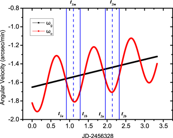
Figure 1. Predicted angular velocity diagram showing the predicted angular velocity of Apophis in both the geocenter and topocenter (IAU O44: Lijiang Station of Yunnan Observatory) from 2013 February 4 to 7. The angular velocities in the geocenter and topocenter are plotted in black and red, respectively. The angular velocity is derived from JPL ephemeris in R.A. t1a and t1b are the times of observation of the two frames obtained on the first night. t2a and t2b are the times of observation of the two frames obtained on the second night. t1m and t2m are the mid-times of observation of frames obtained on the first night and the second night, respectively.
Download figure:
Standard image High-resolution imageFirst, the  value used for calculations in Paper II was not clearly specified. Indeed, Paper II took the geodetic latitude as
  and the Earth radius as ρ. Strictly, the geocentric latitude (
 ) and the distance between the observer and geocenter (ρ) should be used. According to the Explanatory Supplement to the Astronomical Almanac (Seidelmann & Urban 2010),
  and ρ can be accurately calculated using the geodetic longitude, latitude, and altitude of the observatory. For example, as for the location at the Lijiang Station of Yunnan Observatory, ρ and
  (used in this work) are 6377.112 km and 26°32
 28'', respectively, after calculation while the geodetic latitude is 26°41
 43''.
43''.
Second, both Papers I and II elaborate on the errors of ω1 and ω2 (the main errors of ω). This is expressed in Equation (5),

where σα is the standard deviation of the measured R.A. and (tb − ta ) is the difference of the two observation time intervals on the same night. However, due to the change in the relative distances of NEAs, the errors derived from the variable distance of an asteroid r should be considered, which was regarded to be negligible in Papers I and II.
We derive the errors by the change in the distance r. Suppose that the distance of an asteroid changes linearly with time during the observation. Thus, we describe the speed along the distance  . The time interval ΔTm
is the difference between t2m
and t1m
, and rm
is r at the mid-time of t1m
and t2m
. The distances of an asteroid at t1m
and t2m
can be expressed approximately by Equations (6) and (7).
. The time interval ΔTm
is the difference between t2m
and t1m
, and rm
is r at the mid-time of t1m
and t2m
. The distances of an asteroid at t1m
and t2m
can be expressed approximately by Equations (6) and (7).


Considering the conditions above, Equations (6) and (7) in Paper II should be replaced by Equations (8) and (9).

Let  =
=  , which is usually very small (for example, = 0.01). The improved equation of the distance measurement should be Equation (10), in which the change in the distance is considered. The relative errors measured using Equation (2) can be estimated using Equation (11).

In fact, the actual errors will be larger than those estimated using Equation (11) because r and ωg
are not completely linear. To obtain an accurate distance of an asteroid, there are two ways for us to reduce or eliminate the errors from the change in r with the time. The first way is to calculate the value of so that we can measure the distance using the more accurate Equation (10). If we observe an asteroid for more than two nights, for example, for three successive nights, we can measure the distances at the two moments using the observations obtained on the successive two nights according to Equation (2). Using the observations obtained on the first and second nights, we can derive one distance at one moment; using the observations obtained on the second and third nights, we can derive another distance at another moment. Given that the speed along the distance asteroid  is linear with time, we can calculate the approximate
  . Once
  is derived, can be calculated. The second way is to assume
  according to Equation (11), i.e.,

In all cases during the two-night observation, because both  and
and  are greater than 0, the condition above is easily satisfied. However, the best condition is to observe an asteroid at two approximate hour angles. In particular, we should observe the asteroid when H2a
≈ H1a
and H2b
≈ H1b
. According to the assumptions and error estimation, the following factors are the key elements for obtaining the accurate and precise distances of asteroids.
are greater than 0, the condition above is easily satisfied. However, the best condition is to observe an asteroid at two approximate hour angles. In particular, we should observe the asteroid when H2a
≈ H1a
and H2b
≈ H1b
. According to the assumptions and error estimation, the following factors are the key elements for obtaining the accurate and precise distances of asteroids.
- 1.The relative distance changes little (i.e.,
 is small) and linearly.
 - 2.The ωg value of the asteroid changes linearly during observation.
- 3.If we observe an asteroid for more than three nights, we should ensure a longer time interval during one night and use Equation (10) for the distance measurement. If we observe for only two nights, one should follow the hour angle Equation (12) with a time interval as long as possible to reduce the error of ω.

From the derived Equation (10), we know that obtaining the accurate and precise distance does not mean that the asteroid is near its opposition. In fact, we can obtain an even more accurate and precise distance when the object is not near the opposition because ωg is more significantly linear far from its opposition.
Generally, there are two aspects to discuss regarding the differences between this work and previous works (Papers I and II). The first aspect is the different target and case. Previous works found that the RRV method worked well for MBAs, but application to NEAs has not been tapped. In this work, we find that RRV method works well for both MBAs and NEAs. Further, previous works assumed the method only worked near the opposition of an asteroid, while we find that it also works well even if it is not close to the opposition. The second aspect is the improvement in the equation used for distance measurement. We improved the value of  (using the geocentric latitude and the actual distance between the observer and geocenter). We also improved the errors by the change in the distance r (using a more precise equation with or follow the hour angle equation). In Section 4.1, we use the same observation of Apophis and compare the results in this work with the results obtained using the method in Paper II.
3. Observations and Data Reduction
3.1. Observations of Apophis
Apophis is a PHA discovered by Bernardi, Tholen, and Tucker on 2004 June 19 at the Kitt Peak Observatory (Minor Planet Supplement 109613). It had been predicted that there would be an encounter with the Earth on 2029 April 13, with an impact probability of 2.7% , but later it was ruled out (Giorgini et al. 2008; Farnocchia et al. 2013). Some other encounter events were forecast in 2068, 2085, and 2088 (Souchay et al. 2018). Apophis is usually fainter than 20 mag (apparent magnitude) while it can be detected using the stacking method or observing with a large-diameter telescope (Guo et al. 2022). Nevertheless, Wang et al. (2015) and Thuillot et al. (2015) obtained precise astrometric positions when it is much brighter (<17 mag), in the year 2013.
In this work, we reuse the observations of Apophis published by Wang et al. (2015) for distance measurement, which was originally used for position measurement and astrometric calibration. The observations we used in this work were acquired in 2013 February by the 2.4 m telescope at Lijiang Station of Yunnan Observatory (IAU code: O44). The specifications of the telescope and the observations are shown in Tables 1 and 2, respectively. In order to ensure the accuracy of the distance measurement, we use the observations obtained with a large time interval for each night according to Equation (5). In particular, we used the frames observed at the beginning and the end of each night to measure the distance unless the frames were of poor quality. For the observations of each night (see Table 2), a total of 10 frames were used to measure the distance, including 5 frames at the start of observation and 5 frames at the end of observation. The exposure time ranges from 20 to 40 s using the B or I filter in the Johnson–Cousins system. On 2013 February 4, when Apophis was located before the meridian, no frame was observed. On the other three nights, we observed Apophis when it was located before and after the meridian.
Table 1. Specifications of the 2.4 m Telescope at Lijiang Station of Yunnan Observatory and the Attached CCD
| Item | Parameter |
|---|---|
| Geodetic Position | 100°1'51''E, 26°42'32''N |
| Focal Length | 1920 cm |
| Diameter of Primary Mirror | 240 cm |
| F Ratio | 8 |
| CCD Field of View | 9' × 9' |
| Size of Pixel | 13.5 × 13.5 μm |
| Size of CCD Array (Effective) | 1900 × 1900 |
| Approximate Scale Factor | ∼0 286 pixel−1 286 pixel−1
|
Download table as: ASCIITypeset image
Table 2. Observations Used to Measure the Distance of Apophis from 2013 February 4 to 7
| Set Name | Frame ID | Date (UT) | JD | R.A. (h m s) | Decl. (d m s) | Hour Angle (deg) |
|---|---|---|---|---|---|---|
| A1 | A11 | 2013-2-4 | 2456328.15250 | 07 08 21.289 | −06 22 05.33 | 2.6406 |
| A12 | 2013-2-4 | 2456328.15290 | 07 08 21.215 | −06 22 04.22 | 2.7829 | |
| A13 | 2013-2-4 | 2456328.15330 | 07 08 21.142 | −06 22 03.17 | 2.9253 | |
| A14 | 2013-2-4 | 2456328.15369 | 07 08 21.067 | −06 22 02.09 | 3.0718 | |
| A15 | 2013-2-4 | 2456328.15409 | 07 08 20.994 | −06 22 01.01 | 3.2142 | |
| A2 | A21 | 2013-2-4 | 2456328.18531 | 07 08 15.242 | −06 20 36.71 | 14.5064 |
| A22 | 2013-2-4 | 2456328.18577 | 07 08 15.155 | −06 20 35.46 | 14.6739 | |
| A23 | 2013-2-4 | 2456328.18623 | 07 08 15.071 | −06 20 34.22 | 14.8372 | |
| A24 | 2013-2-4 | 2456328.18669 | 07 08 14.987 | −06 20 32.96 | 15.0047 | |
| A25 | 2013-2-4 | 2456328.18715 | 07 08 14.903 | −06 20 31.73 | 15.1721 | |
| B1 | B11 | 2013-2-5 | 2456329.11376 | 07 05 54.831 | −05 39 13.72 | −9.7484 |
| B12 | 2013-2-5 | 2456329.11430 | 07 05 54.735 | −05 39 12.28 | −9.5558 | |
| B13 | 2013-2-5 | 2456329.11482 | 07 05 54.648 | −05 39 10.97 | −9.3674 | |
| B14 | 2013-2-5 | 2456329.11539 | 07 05 54.547 | −05 39 09.38 | −9.1623 | |
| B15 | 2013-2-5 | 2456329.11592 | 07 05 54.452 | −05 39 07.99 | −8.9697 | |
| B2 | B21 | 2013-2-5 | 2456329.24329 | 07 05 32.457 | −05 33 29.15 | 37.1016 |
| B22 | 2013-2-5 | 2456329.24383 | 07 05 32.370 | −05 33 27.79 | 37.2983 | |
| B23 | 2013-2-5 | 2456329.24455 | 07 05 32.248 | −05 33 25.85 | 37.5537 | |
| B24 | 2013-2-5 | 2456329.24514 | 07 05 32.152 | −05 33 24.34 | 37.7714 | |
| B25 | 2013-2-5 | 2456329.24573 | 07 05 32.055 | −05 33 22.76 | 37.9807 | |
| C1 | C11 | 2013-2-6 | 2456330.12909 | 07 03 28.536 | −04 54 42.28 | −2.6223 |
| C12 | 2013-2-6 | 2456330.13006 | 07 03 28.378 | −04 54 39.74 | −2.2706 | |
| C13 | 2013-2-6 | 2456330.13077 | 07 03 28.260 | −04 54 37.88 | −2.0153 | |
| C14 | 2013-2-6 | 2456330.13139 | 07 03 28.159 | −04 54 36.28 | −1.7892 | |
| C15 | 2013-2-6 | 2456330.13212 | 07 03 28.041 | −04 54 34.40 | −1.5255 | |
| C2 | C21 | 2013-2-6 | 2456330.24602 | 07 03 09.604 | −04 49 36.50 | 39.6677 |
| C22 | 2013-2-6 | 2456330.24658 | 07 03 09.514 | −04 49 35.07 | 39.8686 | |
| C23 | 2013-2-6 | 2456330.24730 | 07 03 09.400 | −04 49 33.16 | 40.1281 | |
| C24 | 2013-2-6 | 2456330.24784 | 07 03 09.317 | −04 49 31.77 | 40.3248 | |
| C25 | 2013-2-6 | 2456330.24845 | 07 03 09.221 | −04 49 30.13 | 40.5466 | |
| D1 | D11 | 2013-2-7 | 2456331.07949 | 07 01 22.240 | −04 13 45.19 | −19.0184 |
| D12 | 2013-2-7 | 2456331.08034 | 07 01 22.111 | −04 13 43.05 | −18.7087 | |
| D13 | 2013-2-7 | 2456331.08230 | 07 01 21.807 | −04 13 38.03 | −18.0013 | |
| D14 | 2013-2-7 | 2456331.08290 | 07 01 21.718 | −04 13 36.56 | −17.7837 | |
| D15 | 2013-2-7 | 2456331.08350 | 07 01 21.624 | −04 13 34.96 | −17.5660 | |
| D2 | D21 | 2013-2-7 | 2456331.13431 | 07 01 13.792 | −04 11 25.18 | 0.8083 |
| D22 | 2013-2-7 | 2456331.13503 | 07 01 13.677 | −04 11 23.28 | 1.0678 | |
| D23 | 2013-2-7 | 2456331.13572 | 07 01 13.571 | −04 11 21.47 | 1.3189 | |
| D24 | 2013-2-7 | 2456331.13641 | 07 01 13.462 | −04 11 19.67 | 1.5701 | |
| D25 | 2013-2-7 | 2456331.13708 | 07 01 13.362 | −04 11 18.02 | 1.8087 |
Note. A total of 40 frames were used, and they are shown in eight frame sets. The first and second columns are the set name and frame ID. The third column is the observed date in UT. The fourth column is the mid-exposure time in JD. The fifth and sixth columns are the measured R.A. and decl. of Apophis, respectively, according to Section 3.2. The last column shows the calculated apparent hour angle in degrees.
Download table as: ASCIITypeset image
During our observations, Apophis passed through the galactic belt, and there were enough reference Gaia stars (∼600 Gaia stars could be detected at each frame) for astrometric calibration. It was proximate to the Earth with a distance of ∼0.12 au. The changes in ωg and ωo in R.A. during the observation time according to JPL ephemeris are shown in Figure 1. The ωg value of Apophis changes almost linearly in R.A., and (ωo − ωg ) changes sinusoidally. The mean relative distance on two successive nights is less than 2% (see the left panel of Figure 2). It was not near its opposition, and the solar phase angle was ∼35°.
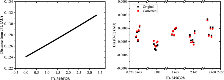
Figure 2. The left panel shows the distance of Apophis with respect to time (from 2013 February 4 to 7) from JPL ephemeris. The right panel shows the difference between the measured and the computed distances from JPL ephemeris (O − C) in au for the independent exposure frames. The black and red spots are the (O − C)s measured using Equations (2) and (10), respectively.
Download figure:
Standard image High-resolution image3.2. Astrometric Data Reduction
Before measuring the distance using Equations (2) or (10), we should derive the observed positions (R.A. and decl.) of the object. Each frame is reduced by the following procedures. First, we derive the pixel position (x, y) for each star and (x0, y0) for the object using a two-dimensional Gaussian centering algorithm. Second, we calculate the standard coordinate (ξ, η) of each star through the central projection (Green 1985). Here, the reference equatorial coordinates (α, δ) are taken from the Gaia Early Data Release 3 catalog (Gaia Collaboration et al. 2021), and stars are calculated to the astrometric positions at the observational epoch. Third, The least squares scheme is used to solve the plate model with a weighted fourth-order polynomial (Lin et al. 2019). Finally, the observed positions of the object can be calculated through the plate model and projection. The observed positions of Apophis used in this work are shown in Table 2.
3.3. Distance Measurement
For the observations in Table 2, we can combine the frames according to the observation time in the following two ways. The first way is to combine each independent exposure frame. In particular, for the five frames of A1 and the five frames of A2 observed on February 4, 2013, we can derive five sets of (t1a , t2a ) s. In chronological order, the five frames of A1 are arranged as A11, A12, A13, A14, A15, and the five frames of A2 are arranged as A21, A22, A23, A24, A25. Then, the five sets of (t1a , t1b )s are (A11, A21), (A12, A22), (A13, A23), (A14, A24), (A15, A25). In the same way, the five sets of (t2a , t2b )s can be defined as (B11, B21), (B12, B22), (B13, B23), (B14, B24), (B15, B25). By combining the frame sets (A1, A2, B1, and B2) according to the arrangement order (combination of (A11, A21) and (B11, B21), (A12, A22) and (B12, B22), ⋯), the five distance results of the object can be obtained. In this way, 30 distance results of the object can be obtained, including 15 distance results from the frames observed on there successive two nights, 10 distance results from the frames observed two nights apart, and five distance results from the frames observed three nights apart. Another way is to calculate the mean positions for each set of observations in Table 2. In particular, we calculate the mean observed positions, time, and hour angles for each frame set. Each set in Table 2 is regarded as an independent exposure frame. Then, six distance results can be obtained, including three distance results from the successive two nights, two distance results from two nonsuccessive nights, and one result from three nonsuccessive nights.
For each frame, the observation time was recorded during the observation, and the hour angle could be calculated. The observed positions (R.A. and decl.) of the object can be calculated according to the procedures in Section 3.2. As the distance results we calculated are the mean distances at t1a
, t1b
, t2a
, and t2b
, the decl. of the object we used to calculate  is the mean decl. of the four observed moments at t1a
, t1b
, t2a
, and t2b
. After we derive the distance, we compare our results with JPL ephemeris, from which the distance is computed at the mean time of t1a
, t1b
, t2a
, and t2b
. The results and further analysis are presented in Section 4.
is the mean decl. of the four observed moments at t1a
, t1b
, t2a
, and t2b
. After we derive the distance, we compare our results with JPL ephemeris, from which the distance is computed at the mean time of t1a
, t1b
, t2a
, and t2b
. The results and further analysis are presented in Section 4.
4. Results and Discussion
4.1. Distance Results
The calculated distance results of Apophis for the independent exposure frames (the first way described in Section 3.3) are shown in Tables 3 and 5. The calculated distance results for the mean positions of each set of observations (the second way described in Section 3.3) are shown in Table 6. The time intervals for ΔT1 (the difference of t1b
and t1a
), ΔT2 (the difference of t2b
and t2a
) and ΔTm
(the difference of t2m
and t1m
) are shown in the result tables. We compare the distances of Apophis measured using three methods, including using Equations (2) and (10) and the method in Paper II. After we calculate the distances for two nights (observations for three nights), the speed along the distance  can be also derived. Thus, we can measure the distances by a more accurate Equation (10). The difference of the measured distances (the observed) minus the distances from JPL ephemeris (the computed) as well as its relative errors are also given. From the distance results for using independent exposure frames on the successive two nights, the observations for date 0205–0206 (the observations on February 5 are calculated as t1 and the observations on February 6 are calculated as t2) show lower errors. This is mainly because of the larger time interval on ΔT1 and ΔT2. A smaller time interval will cause larger errors of ωg
according to Equation (5). In contrast, the observations for dates 0204–0205 and 0206–0207 with shorter time intervals of ΔT1 and ΔT2 have larger relative errors. With the calculated speed along the distance, the total mean relative error for the independent frames obtained on the successive two nights is 0.080% (0.000068 au), while the relative error using the method in Paper II is 0.179%. The results in this work have about a factor of 2 improvement compared with the results using the method in Paper II. For the results of the observations obtained on two nights apart and three nights apart, the relative errors are larger compared with the results of the frames obtained on the successive two nights. Their mean total results are 0.234% (0.000298 au) and 0.511% (0.000652 au), respectively. The results measured using Equations (2) or (10) show that the interval of ΔTm
affects the accuracy, which is mainly related to the not completely linear change in the distance in a larger time span. Take Apophis as an example and suppose the distance of Apophis is a quadratic function with time. We fit the quadratic function near the time when the distance of Apophis is the maximum or minimum (in the case the curvatures are larger) to the Earth according to JPL ephemeris in 2013. In this way, we calculate the measured errors of distance assuming a linear relation of the distance with time. We find it relevant to the curvature K and ΔTm
(ΔTm
= 1 means using the observations obtained on the successive two nights, and ΔTm
= 2 means using those obtained two nights apart). Table 7 shows the errors in different cases. Generally, we find that this error is 0.000028 au for a curvature K of 0.00022 using the observations obtained on the successive two nights. This error would become larger with an increase in ΔTm
. However, the actual curvature is hard to be derived from observations made on nonsuccessive nights. Therefore, to accurately calculate the distance, we should use observations obtained on successive nights.
can be also derived. Thus, we can measure the distances by a more accurate Equation (10). The difference of the measured distances (the observed) minus the distances from JPL ephemeris (the computed) as well as its relative errors are also given. From the distance results for using independent exposure frames on the successive two nights, the observations for date 0205–0206 (the observations on February 5 are calculated as t1 and the observations on February 6 are calculated as t2) show lower errors. This is mainly because of the larger time interval on ΔT1 and ΔT2. A smaller time interval will cause larger errors of ωg
according to Equation (5). In contrast, the observations for dates 0204–0205 and 0206–0207 with shorter time intervals of ΔT1 and ΔT2 have larger relative errors. With the calculated speed along the distance, the total mean relative error for the independent frames obtained on the successive two nights is 0.080% (0.000068 au), while the relative error using the method in Paper II is 0.179%. The results in this work have about a factor of 2 improvement compared with the results using the method in Paper II. For the results of the observations obtained on two nights apart and three nights apart, the relative errors are larger compared with the results of the frames obtained on the successive two nights. Their mean total results are 0.234% (0.000298 au) and 0.511% (0.000652 au), respectively. The results measured using Equations (2) or (10) show that the interval of ΔTm
affects the accuracy, which is mainly related to the not completely linear change in the distance in a larger time span. Take Apophis as an example and suppose the distance of Apophis is a quadratic function with time. We fit the quadratic function near the time when the distance of Apophis is the maximum or minimum (in the case the curvatures are larger) to the Earth according to JPL ephemeris in 2013. In this way, we calculate the measured errors of distance assuming a linear relation of the distance with time. We find it relevant to the curvature K and ΔTm
(ΔTm
= 1 means using the observations obtained on the successive two nights, and ΔTm
= 2 means using those obtained two nights apart). Table 7 shows the errors in different cases. Generally, we find that this error is 0.000028 au for a curvature K of 0.00022 using the observations obtained on the successive two nights. This error would become larger with an increase in ΔTm
. However, the actual curvature is hard to be derived from observations made on nonsuccessive nights. Therefore, to accurately calculate the distance, we should use observations obtained on successive nights.
Table 3. Distance Results of Apophis Using Independent Frames Obtained on The Successive Two Nights
| Date | ΔT1 | ΔT2 | ΔTm | JPL_r | (O − C)_r1 | (O − C)_r2 | (O − C)_paper2 | Err_r1 | Err_r2 | Err_paper2 |
|---|---|---|---|---|---|---|---|---|---|---|
| (h) | (h) | (JD) | (au) | (au) | (au) | (au) | (%) | (%) | (%) | |
| 0204-0205 | 0.78744 | 3.10867 | 1.009619 | 0.125547 | −0.000205 | −0.000179 | −0.000353 | 0.163 | 0.143 | 0.281 |
| 0204-0205 | 0.78898 | 3.10884 | 1.009729 | 0.125548 | −0.000092 | −0.000066 | −0.000240 | 0.073 | 0.053 | 0.191 |
| 0204-0205 | 0.79046 | 3.11330 | 1.009921 | 0.125549 | −0.000285 | −0.000259 | −0.000433 | 0.227 | 0.206 | 0.345 |
| 0204-0205 | 0.79186 | 3.11417 | 1.010076 | 0.125550 | −0.000069 | −0.000042 | −0.000217 | 0.055 | 0.034 | 0.173 |
| 0204-0205 | 0.79339 | 3.11525 | 1.010205 | 0.125551 | 0.000035 | 0.000062 | −0.000113 | 0.028 | 0.049 | 0.090 |
| 0204-0205 | Mean | 0.125549 | −0.000123 | −0.000097 | −0.000353 | 0.109 | 0.097 | 0.216 | ||
| 0205-0206 | 3.10867 | 2.80630 | 1.009031 | 0.127771 | −0.000144 | −0.000133 | −0.000295 | 0.113 | 0.104 | 0.231 |
| 0205-0206 | 3.10884 | 2.79641 | 1.009253 | 0.127773 | −0.000073 | −0.000061 | −0.000224 | 0.057 | 0.048 | 0.175 |
| 0205-0206 | 3.11330 | 2.79670 | 1.009347 | 0.127774 | −0.000161 | −0.000149 | −0.000312 | 0.126 | 0.117 | 0.244 |
| 0205-0206 | 3.11417 | 2.79480 | 1.009351 | 0.127776 | −0.000016 | −0.000003 | −0.000167 | 0.012 | 0.003 | 0.130 |
| 0205-0206 | 3.11525 | 2.79197 | 1.009462 | 0.127777 | 0.000004 | 0.000017 | −0.000147 | 0.003 | 0.013 | 0.115 |
| 0205-0206 | Mean | 0.127774 | −0.000078 | −0.000066 | −0.000229 | 0.062 | 0.057 | 0.179 | ||
| 0206-0207 | 2.80630 | 1.31587 | 0.919344 | 0.129960 | 0.000205 | 0.000176 | 0.000051 | 0.158 | 0.136 | 0.039 |
| 0206-0207 | 2.79641 | 1.31256 | 0.919370 | 0.129962 | −0.000140 | −0.000169 | −0.000293 | 0.108 | 0.130 | 0.226 |
| 0206-0207 | 2.79670 | 1.28213 | 0.919978 | 0.129964 | 0.000024 | −0.000007 | −0.000130 | 0.018 | 0.006 | 0.100 |
| 0206-0207 | 2.79480 | 1.28438 | 0.920038 | 0.129966 | −0.000161 | −0.000193 | −0.000314 | 0.124 | 0.148 | 0.242 |
| 0206-0207 | 2.79197 | 1.28599 | 0.920002 | 0.129967 | 0.000022 | −0.000011 | −0.000132 | 0.017 | 0.009 | 0.102 |
| 0206-0207 | Mean | 0.129963 | −0.000010 | −0.000041 | −0.000164 | 0.085 | 0.086 | 0.142 | ||
| Total Mean | 0.127762 | −0.000070 | −0.000068 | −0.000249 | 0.085 | 0.080 | 0.179 | |||
Note. The specifications are as follows (same for Tables 4 and 6). The first column is the date the frames used for distance measurement were obtained. For example, 0204-0205 means that the observations on February 4 correspond to t1 and the observations on February 5 correspond to t2. The second and the third columns show the differences in the observed time at t1b and t1a as well as t2b and t2a , respectively. The fourth column shows the difference in the observed time at t2m and t1m . The fifth column shows the computed distance from JPL ephemeris. Columns six to eight show the results of the observed (using Equations (2) and (10) and the method in Paper II, respectively) minus the computed distances. The last three columns show the relative errors of the results corresponding to columns six to eight, respectively.
Download table as: ASCIITypeset image
Table 4. Distance Results of Apophis Using the Observations Obtained Two Nights Apart
| Date | ΔT1 | ΔT2 | ΔTm | JPL_r | (O − C)_r1 | (O − C)_r2 | (O − C)_paper2 | Err_r1 | Err_r2 | Err_paper2 |
|---|---|---|---|---|---|---|---|---|---|---|
| (h) | (h) | (JD) | (au) | (au) | (au) | (au) | (%) | (%) | (%) | |
| 0204-0206 | 0.78744 | 2.80630 | 2.018650 | 0.126650 | −0.000355 | −0.000281 | −0.000504 | 0.280 | 0.222 | 0.398 |
| 0204-0206 | 0.78898 | 2.79641 | 2.018981 | 0.126651 | −0.000463 | −0.000388 | −0.000612 | 0.365 | 0.306 | 0.483 |
| 0204-0206 | 0.79046 | 2.79670 | 2.019269 | 0.126653 | −0.000488 | −0.000411 | −0.000637 | 0.385 | 0.325 | 0.503 |
| 0204-0206 | 0.79186 | 2.79480 | 2.019427 | 0.126654 | −0.000398 | −0.000320 | −0.000547 | 0.314 | 0.253 | 0.432 |
| 0204-0206 | 0.79339 | 2.79197 | 2.109667 | 0.126655 | −0.000374 | −0.000296 | −0.000523 | 0.296 | 0.233 | 0.413 |
| 0204-0206 | Mean | 0.126653 | −0.000416 | 0.000339 | −0.000565 | 0.328 | 0.268 | 0.446 | ||
| 0205-0207 | 3.10867 | 1.31587 | 1.928374 | 0.128807 | −0.000148 | −0.000190 | −0.000300 | 0.115 | 0.147 | 0.233 |
| 0205-0207 | 3.10884 | 1.31256 | 1.928623 | 0.128809 | −0.000272 | −0.000315 | −0.000424 | 0.211 | 0.245 | 0.329 |
| 0205-0207 | 3.11330 | 1.28213 | 1.929325 | 0.128811 | −0.000258 | −0.000304 | −0.000410 | 0.200 | 0.236 | 0.318 |
| 0205-0207 | 3.11417 | 1.28438 | 1.929389 | 0.128812 | −0.000319 | −0.000367 | −0.000471 | 0.248 | 0.285 | 0.366 |
| 0205-0207 | 3.11525 | 1.28599 | 1.929464 | 0.128814 | −0.000061 | −0.000111 | −0.000213 | 0.048 | 0.086 | 0.166 |
| 0205-0207 | Mean | 0.128811 | −0.000212 | −0.000257 | −0.000364 | 0.164 | 0.200 | 0.282 | ||
| Total Mean | 0.127732 | −0.000314 | −0.000298 | −0.000464 | 0.246 | 0.234 | 0.364 | |||
Download table as: ASCIITypeset image
Table 5. Distance Results of Apophis Using the Observations Obtained Three Nights Apart
| Date | ΔT1 | ΔT2 | ΔTm | JPL_r | (O − C)_r1 | (O − C)_r2 | (O − C)_paper2 | Err_r1 | Err_r2 | Err_paper2 |
|---|---|---|---|---|---|---|---|---|---|---|
| (h) | (h) | (JD) | (au) | (au) | (au) | (au) | (%) | (%) | (%) | |
| 0204-0207 | 0.78744 | 1.31587 | 2.937994 | 0.127670 | −0.000483 | −0.000475 | −0.000633 | 0.378 | 0.372 | 0.496 |
| 0204-0207 | 0.78898 | 1.31256 | 2.938351 | 0.127672 | −0.000767 | −0.000761 | −0.000917 | 0.601 | 0.596 | 0.718 |
| 0204-0207 | 0.79046 | 1.28213 | 2.939247 | 0.127674 | −0.000690 | −0.000687 | −0.000840 | 0.540 | 0.538 | 0.658 |
| 0204-0207 | 0.79186 | 1.28438 | 2.939465 | 0.127675 | −0.000795 | −0.000794 | −0.000945 | 0.623 | 0.622 | 0.740 |
| 0204-0207 | 0.79339 | 1.28599 | 2.939669 | 0.127676 | −0.000543 | −0.000543 | −0.000693 | 0.425 | 0.425 | 0.543 |
| Total Mean | 0.127674 | −0.000656 | −0.000652 | −0.000806 | 0.513 | 0.511 | 0.631 | |||
Download table as: ASCIITypeset image
Table 6. Distance Results of Apophis Using the Mean Positions for Each Observation Set in Table 2
| Date | ΔT1 | ΔT2 | ΔTm | JPL_r | (O − C)_r1 | (O − C)_r2 | (O − C)_paper2 | Err_r1 | Err_r2 | Err_paper2 |
|---|---|---|---|---|---|---|---|---|---|---|
| (h) | (h) | (JD) | (au) | (au) | (au) | (au) | (%) | (%) | (%) | |
| 0204-0205 | 0.79042 | 3.11206 | 1.009910 | 0.125549 | −0.000122 | −0.000096 | −0.000270 | 0.097 | 0.076 | 0.215 |
| 0205-0206 | 3.11206 | 2.79725 | 1.009289 | 0.127774 | −0.000076 | −0.000064 | −0.000227 | 0.060 | 0.050 | 0.178 |
| 0206-0207 | 2.79725 | 1.29619 | 0.919746 | 0.129964 | −0.000006 | −0.000037 | −0.000160 | 0.005 | 0.028 | 0.123 |
| 0204-0206 | 0.79042 | 2.79725 | 2.019199 | 0.126653 | −0.000414 | −0.000338 | −0.000563 | 0.327 | 0.267 | 0.444 |
| 0205-0207 | 3.11206 | 1.29619 | 1.929035 | 0.128811 | −0.000208 | −0.000254 | −0.000360 | 0.161 | 0.197 | 0.279 |
| 0204-0207 | 0.79042 | 1.29619 | 2.938945 | 0.127673 | −0.000652 | −0.000649 | −0.000802 | 0.511 | 0.508 | 0.628 |
Download table as: ASCIITypeset image
Table 7. Measured Errors of Distance in au for Different Curvatures K and ΔTm
| K | ΔTm = 1 (day) | ΔTm = 2 (day) | ΔTm = 3 (day) | ΔTm = 4 (day) | ΔTm = 5 (day) |
|---|---|---|---|---|---|
| 5.5 × 10⁻⁵ | 6.9 × 10⁻⁶ | 2.8 × 10⁻⁵ | 6.2 × 10⁻⁵ | 1.1 × 10⁻⁴ | 1.7 × 10⁻⁴ |
| 7.7 × 10⁻⁵ | 9.6 × 10⁻⁶ | 3.9 × 10⁻⁵ | 8.7 × 10⁻⁵ | 1.5 × 10⁻⁴ | 2.4 × 10⁻⁴ |
| 9.8 × 10⁻⁵ | 1.2 × 10⁻⁵ | 4.9 × 10⁻⁵ | 1.1 × 10⁻⁴ | 2.0 × 10⁻⁴ | 3.1 × 10⁻⁴ |
| 2.2 × 10⁻⁴ | 2.8 × 10⁻⁵ | 1.1 × 10⁻⁴ | 2.5 × 10⁻⁴ | 4.4 × 10⁻⁴ | 6.9 × 10⁻⁴ |
Download table as: ASCIITypeset image
The results of the mean positions for each observation set in Table 2 have smaller relative errors compared with the mean total results to the corresponding observations. The observations for the date 0204–0207 have the largest relative errors of 0.508% (0.000649 au) compared with other observation sets. For the independent exposure frames, the right panel of Figure 2 shows the difference between the observed (the one we have measured) and the computed (from the JPL ephemeris) distance changes with respect to time. In order to clearly show the different results of using Equations (2) and (10), a total of 25 measured distance results are plotted, including 15 measured results observed on two successive nights and 10 measured results observed two nights apart. The original results measured using Equation (2) are plotted in black while the corrected results measured using Equation (10) are plotted in red. From the right panel of Figure 2, the measured results near the values of 1.18 and 2.14 in the x-axis have larger deviations compared with JPL ephemeris, which are caused by the larger ΔTm of about 2. While other results (near the values of 0.67, 1.68, and 2.65 in the x-axis) have smaller deviations with ΔTm values of about 1. At the time when we observed Apophis, it was far away from us moving at a speed of ∼0.002 au per day. The accuracy of our measurements determined from independent exposure frames obtained on the successive two nights is 0.000068 au, which is sufficient for monitoring the change in distance.
4.2. Simulations
According to the requirement of the RRV method, we simulated the distance measurement of NEAs at the time they were discovered. As we know, NEAs are divided into four groups (Amors, Apollos, Atens, and Atiras) according to their perihelion distances, aphelion distances, and semimajor axes of their orbits. We select the typical four NEAs, (1221) Amor, (1862) Apollo, (2062) Aten, and (163693) Atira, for simulation at their discovery dates and follow-up dates. The positions at the successive two nights (the discovery night and the following night) from JPL ephemeris are used after adding Gaussian noise. The standard deviation of the added Gaussian noise is 002 for both R.A. and decl. The time intervals ΔT1 and ΔT2 are both 1 hr. We suppose that observations were made by the 2.4 m telescope at Lijiang Station of Yunnan Observatory (details in Table 1). The results simulated for 10,000 iterations are shown in Figure 3 for each NEA. We find that δ is insensitive to the distance results, and the difference of the relative distance is usually less than 0.01% when δ is 1 arc minute different from the mean δ (at t1a
, t1b
, t2a
, and t2b
). From the simulation results, we can obtain the accurate and precise distance of each NEA. The mean relative distance values of NEAs (1221) Amor, (1862) Apollo, (2062) Aten, and (163693) Atira are −0.0003 (−0.03%), −0.0140 (−1.40%), −0.0002 (−0.02%), and 0.0019 (0.19%), respectively. Their precision (the standard deviation of the mean relative distance) is estimated at 0.0013 (0.13%), 0.0020 (0.20%), 0.0015 (0.15%), and 0.0118 (1.18%).

Figure 3. The four panels show the simulation results for the NEAs (1221) Amor, (1862) Apollo, (2062) Aten, and (163693) Atira. The blue line is the fitted Gaussian curve according to the distributions of the histogram. Each NEA is simulated for 10,000 iterations. The object name, the added Gaussian noises (assuming that the standard deviations in both R.A. and decl. are 002), the simulated mean relative distance, and the standard deviation of the relative distance are shown above each panel.
Download figure:
Standard image High-resolution image
4.3. Discussion
To measure the distances of NEAs using the RRV method, we do not need to strictly observe the object when it is located before and after the meridian during each night. Further, we do not need to observe the object when it is near its opposition. For the observations of Apophis on February 4, it is only observed when it is located after the meridian with a short time interval of ∼0.8 hr. Nevertheless, we can also obtain accurate distances from observations made on February 4 and 5. The distances can be measured using observations make on several nonsuccessive nights (for example, two or three nights apart) and of course the measurement accuracy is somewhat worse than using the observations obtained on the successive two nights. For these observations, the errors of the measured distance are mainly related to ΔT1, ΔT2, and ΔTm (a not completely linear change in ωg and the distance). To obtain more a accurate distance of Apophis, we should make ΔT1 and ΔT2 larger (on the premise of ensuring the observed position accuracy) and observe the object on successive nights. This method is not so demanding in terms of weather conditions. For example, even if we observe the object only after midnight on one night, and then we observe the same object on the third night (no observations on the second night), we can still measure its distance. For those NEAs within the orbit of the Earth, they might be observed in a short time (e.g., 1 hr). The simulation results of NEAs well reflects this situation, in which we can also obtain accurate and precise distances. From Table 5, we only use the frames observed on the first night with a time interval of ∼0.8 hr and the frames observed on the fourth night with a time interval of ∼1.3 hr for measurement. We can also derive the accurate distance with a mean relative error of 0.513% (0.000656 au) using short time intervals from observations made three nights apart.
Generally, we can derive the accurate and precise distances of NEAs for most cases using this method through observations made over only two nights. For newly discovered asteroids, we can determine whether a certain asteroid is approaching or moving away from us using observations made over only three nights, which is important for impact defense. If we also perform photometry, the absolute magnitude and size of the asteroid can be calculated (given an estimated albedo). Then, the impact risk can be evaluated according to its distance and size. Continuously monitoring the distances of NEAs (especially PHAs) is significant to their orbital improvement and evolution. More importantly, it is promising for Earth security and defense.
5. Conclusion
In this work, we refined the RRV method and extend it further to the distance measurement of NEAs. This method can accurately and precisely measure the distances of MBAs and NEAs for most cases in an astrometric way without performing orbital determination. This method is not demanding for the positions of asteroids themselves, nor the time coordination or the location of the ground-based telescope. We can measure the distance of an asteroid when it is not near its opposition. In practice, we measure the distance of the PHA Apophis from the acquired CCD frames. Using 40 frames over four nights (10 frames per night), our results show that the total mean relative error for the independent exposure frames obtained on the successive two nights is ∼0.08% (about a factor of 2 improvement in comparison with that in Paper II). We also simulate the distance measurement for the four typical NEAs, Amor, Apollo, Aten, and Atira, at their discovery dates and follow-up dates. The simulation results are accurate and precise for observation time intervals of 1 hr each night. The simulation results show that, for the newly discovered asteroids, we can also derive the accurate and precise distances even if they are observed with a short time. The accurate and precise distances of NEAs computed using this method are important for the study of the dynamics and evolution of the solar system. More importantly, it is promising for Earth security and defense.
We are grateful for the group of the 2.4 m telescope of Lijiang Station, Yunnan Observatory who assisted in obtaining observations. We also deeply thank Prof. Zi Zhu and Dr. Hong Zhang from Nanjing University for valuable discussions with us. Also, we thank Ying Chen, Yaoyao Hong, Jianan Hao, Zhongjie Zheng, Xiao Chen, and Xueqing Fang for their help. This research is supported by the Key Special Project of the Ministry of the National Science and Technology (grant No. 2022YFE0116800), by the National Natural Science Foundation of China (grant Nos.11873026, 11273014, 12203019), by the Joint Research Fund in Astronomy (grant No.U1431227), by the science research grants from the China Manned Space Project with NO. CMS-CSST-2021-B08 and Excellent Postgraduate Recommendation Scientific Research Innovative Cultivation Program of Jinan University. This work has made use of data from the European Space Agency (ESA) mission Gaia (https://www.cosmos.esa.int/gaia), processed by the Gaia Data Processing and Analysis Consortium (DPAC; https://www.cosmos.esa.int/web/gaia/dpac/consortium). Funding for the DPAC has been provided by national institutions, in particular the institutions participating in the Gaia Multilateral Agreement.
Footnotes
- 4
- 5