


Abstract
Using data from the Arecibo Galaxy Environment Survey, we report the discovery of five H i clouds in the Leo I group without detected optical counterparts. Three of the clouds are found midway between M96 and M95, one is only from the southeast side of the well-known Leo Ring, and the fifth is relatively isolated. H i masses range from 2.6 × 10⁶ M⊙ to 9.0 × 10⁶ M⊙, and velocity widths (W50) range from 16 to 42 km s−1. Although a tidal origin is the most obvious explanation, this formation mechanism faces several challenges. For the most isolated cloud, the difficulties are its distance from neighboring galaxies and the lack of any signs of disturbance in the H i disks of those systems. Some of the clouds also appear to follow the baryonic Tully–Fisher relation between mass and velocity width for normal, stable galaxies, which is not expected if they are tidal in origin. Three clouds are found between M96 and M95 that have no optical counterparts but have otherwise similar properties and locations to the optically detected galaxy LeG 13. While overall we favor a tidal debris scenario to explain the clouds, we cannot rule out a primordial origin. If the clouds were produced in the same event that gave rise to the Leo Ring, they may provide important constraints on any model attempting to explain that structure.


Original content from this work may be used under the terms of the Creative Commons Attribution 4.0 licence. Any further distribution of this work must maintain attribution to the author(s) and the title of the work, journal citation and DOI.
1. Introduction
The Leo I group is well known for its numerous optically dark H i features. At approximately 11 Mpc distance, the group consists of at least four major galaxies. Its most unusual feature is the spectacular Leo Ring, a 225 kpc diameter arc of approximately 1.7 × 10⁹ M⊙ of H i (Schneider 1989; Stierwalt et al. 2009). Some isolated patches of optical emission have been detected at various points within the Ring (Thilker et al. 2009), but on the large scale the H i has no associated optical component. The origin of this structure is still unclear. It has been suggested to be primordial (Schneider 1989; Sil'chenko et al. 2003), though metallicity measurements suggest otherwise (Rosenberg et al. 2014; Corbelli et al. 2021). One alternative explanation is a galaxy–galaxy collision (Michel-Dansac et al. 2010), which well reproduces the overall morphology but has difficulties explaining the observed kinematics.
At approximately the same location on the sky as some parts of the Ring, but at a higher velocity, extended H i emission is also seen around the galaxy NGC 3389 (Stierwalt et al. 2009). This feature, although less dramatic, itself still extends across ∼90 kpc. It contains several optically bright galaxies and appears relatively easy to explain by tidal interactions. Elsewhere in Leo, the Leo Triplet contains a ∼100 kpc H i plume (Stierwalt et al. 2009), while even larger features are reported in Leisman et al. (2016).
Giant, elongated H i structures are often easily explained by galaxy–galaxy interactions (e.g., Toomre & Toomre 1972; Bekki et al. 2005; Duc & Bournaud 2008; Taylor et al. 2017) or ram pressure stripping (Oosterloo & van Gorkom 2005; Tonnesen & Bryan 2010; Taylor et al. 2020). Less common are small, discrete H i clouds with no obvious extended feature to indicate their parent galaxy—we describe a few of these in Section 4.6, with a longer review given in Taylor et al. (2016). The origin of such clouds tends to be controversial. While they may be the remnants of dispersed streams from tidal encounters, an alternative is that they are dark-matter-dominated but extremely dim (or even entirely dark) galaxies, either primordial (Davies et al. 2004; Minchin et al. 2007) or resulting from interactions (Román et al. 2021).
We tested these explanations in Taylor et al. (2016) and Taylor et al. (2017). We found that the majority of cases of such isolated clouds can indeed be explained as tidal debris, as may particular features embedded within larger structures, such as VIRGOHI21 (Haynes et al. 2007; Minchin et al. 2007). In contrast, we also showed that while our simulations readily produced isolated clouds of low velocity widths (<50 km s−1), clouds of line width >100 km s−1 were virtually nonexistent in those same simulations. This makes the clouds described in Taylor et al. (2012) and Taylor et al. (2013) particularly challenging to explain.
In this paper we present the discovery of five new clouds in the Leo I region using a deep Arecibo survey. While a handful of such clouds are known in other groups, this is the first time such clouds have been found in this environment. We discuss the possible origin of the clouds, considering the strengths and weaknesses of different models proposed to explain the formation of the Leo Ring.
The rest of this paper is organized as follows. In Section 2 we describe the observations, data reduction, and source extraction of the H i data used in this analysis. The results are presented in Section 3 and analyzed in Section 4. Finally, we summarize our findings in Section 5. Throughout, we assume a group distance of 11.1 Mpc following Stierwalt et al. (2009). At this distance, the Arecibo 3 5-diameter beam has a physical size of 11.3 kpc. Stierwalt et al. (2009) give the group velocity dispersion as 175 km s−1. Since all of our clouds have systemic velocities within 75 km s−1 of M96, we assume that they are all at the group distance of 11.1 Mpc unless stated otherwise.
2. Observations
2.1. The AGES Data
The Arecibo Galaxy Environment Survey (AGES; Auld et al. 2006) was a blind H i survey performed at the Arecibo radio telescope from 2006 to 2019. This was part of a tiered approach to H i surveys taking advantage of the then-new Arecibo L-band Feed Array (ALFA) receiver. To this end, the Arecibo Legacy Fast ALFA survey (ALFALFA; Giovanelli et al. 2005) covered approximately 7000 deg2 to an rms sensitivity of about 2.2 mJy, AGES provides a medium-deep survey of 200 deg2 to 0.7 mJy, and the Arecibo Ultra Deep Survey (AUDS; Xi et al. 2021) examined 1.4 deg2 to 0.08 mJy rms. AGES targeted the full range of galaxy environments from voids to clusters, with one of the major goals being the detection of optically dark H i sources that could not be discovered by optical surveys. The 1σ column density sensitivity of AGES is = 1.5 × 1017 cm−2 (0.001 M⊙ pc−2) for a source that fills the beam at 10 km s−1 velocity resolution (Keenan et al. 2016); while AGES has a maximum velocity resolution of 5 km s−1, we Hanning-smooth the data to 10 km s−1 for better sensitivity and reduction of artifacts such as Gibbs ringing.

The AGES observing strategy and data reduction techniques have been described in detail in Auld et al. (2006), Minchin et al. (2010), and Davies et al. (2011). They are here only summarized. AGES was a fixed-azimuth drift scan survey. The telescope was pointed to the start position of a scan and the sky allowed to drift overhead, typically for 20 minutes (as here) to cover 5° of R.A. with the seven beams of the ALFA receiver. Each point took about 12 s to cross the beam. When complete, the telescope was reoriented to the next scan, staggered by one-third of the beam size (35) to create a fully Nyquist-sampled map. The total on-source integration time per point was 300 s.
Observations of the Leo field were carried out in 2012 (January–February, November–December), 2013 (February, April–May, November–December), 2014 (January), 2015 (January–March, May, December), 2016 (December), 2017 (January–February), 2018 (January–May, December), and 2019 (January). The observations cover a field of approximately 5° of R.A. and 4° of decl., centered on 10:45:00, 12:48:00. The full range of the field is 10:34:49–10:55:14 in R.A. and 10:42:58–14:52:01 in decl. The bandwidth covered is equivalent in heliocentric velocity from −2000 to +20,000 km s−1. Due to the hexagonal beam pattern of ALFA, sensitivity is reduced over a few arcminutes near the spatial edges of the field. Sensitivity is also reduced over the final 1000 km s−1 of spectral baseline. We are here only presenting observations of the M96 subgroup, which is in a frequency range unaffected by interference.
The data from the two linear polarizations for each of ALFA's seven beams are reduced using the livedata and gridzilla software packages. Following Taylor et al. (2014), we further apply a second-order polynomial to the spectra at every pixel in the resulting data cube, further reducing the impact of continuum sources. Additionally, we apply a medmed (Putman et al. 2002) correction to each spatial baseline. This divides each baseline into five equal segments, computes the median value of the flux in each one, and then subtracts the median of the medians. The advantage of this is a significant reduction in "shadows" in the data, caused by oversubtraction of bright extended sources (an example is shown in Minchin et al. 2010).
2.2. Source Extraction
We here concentrate on the primary target region, the M96 subgroup in Leo. The primary target for AGES in this region was the Leo Ring. In the course of investigating this feature, we serendipitously discovered several discrete H i clouds that are optically undetected (we refer to them as "dark" by convention; see Section 3.2 for details), at least one of which appears to have no association with the Ring. We restrict our present analysis to these clouds and leave discussion of the Ring itself, as well as a catalog over the full AGES spectral bandwidth, to future works. Here we limit our search to the M96 subgroup, within the velocity range 300–1600 km s−1. All of the clouds are within 75 km s−1 of the velocity of M96.
We searched the full spatial field by eye using the FRELLED software described in Taylor (2015). While this has been considerably updated since its initial release, to be described in a future paper, the basic source extraction procedure remains the same (see, e.g., Taylor et al. 2014). We first display the cube in a volume render, defining masks around anything that visually resembles an H i source. The advantage of the volume rendering technique is that it enables very rapid masking, since the user can see the 3D (velocity space) structure of the source at a glance. The downside is that this often makes the faintest sources hard to detect. We therefore proceed to a second stage. With the masks still hiding the sources already found, we search each individual slice (i.e., channels and position–velocity (PV) slices) of the data cube and apply additional masks if any more sources are detected—in this case, no further sources were found. This approach is designed to combine the key advantages of the rapid cataloging speed enabled through volumetric rendering, together with the sensitivity of more traditional visualization techniques.
We quantify the H i parameters of each detection using the miriad package mbspect (Sault et al. 1995). We define the spectral profile window by eye, and mbspect applies position fitting by computing the centroid of a 2D Gaussian to the integrated map over the specified velocity range. It then computes the total integrated flux (SH i ) and velocity width at 50% (W50) and 20% (W20) of the peak flux. The H i mass is computed by the standard equation:

We searched for optical counterparts by checking the Sloan Digital Sky Survey (SDSS) and NASA Extragalactic Database (NED) at the position-fitted coordinates of the source, searching within a 17 (half the FWHM) radius and checking whether any visible or listed sources have optical redshift measurements within 200 km s−1 of the H i measurement. These search parameters are deliberately very generous to maximize the chance of finding any plausible optical counterpart. Typically, from other AGES data sets (e.g., Taylor et al. 2012) optical counterparts have spatial positions within about 20'' of the H i coordinates; the resolution of the survey is usually more than sufficient for identifying any counterparts where they exist. Similarly, the difference between optical and H i redshifts for candidate optical counterparts is usually less than 50 km s−1.
Quantifying the H i mass sensitivity is complicated, as the signal-to-noise ratio (S/N) level for a source of a given mass varies according to both its line width and peak flux: no matter how massive, at a sufficiently high line width a source will always become so faint as to be undetectable. As a rough estimate, a source of 4σ with top-hat profile of width 50 km s−1 is a reasonable approximation for the faintest readily detectable source, which at 11.1 Mpc corresponds to an H i mass of 4.1 × 10⁶ M⊙. Some of the sources presented here have masses close to or even below this value, raising the issue as to whether our source extraction is complete for clouds of the given parameters. But a top-hat profile is not realistic. A more sophisticated sensitivity estimate can be provided using the Saintonge (2007) definition of integrated S/N, which accounts for the variation in line width and peak flux together. ALFALFA is reckoned to be complete for total S/N values, by this definition, above 6.5. By injecting several thousand artificial sources of different line widths and fluxes into galaxy-free data cubes and running our own source extraction procedures, we show that AGES completeness well matches the ALFALFA criteria (R. Taylor et al. 2022, in preparation). All of the clouds presented herein have total S/N values exceeding 6.5, showing that we are indeed complete for clouds similar to those we detect.
3. Results
3.1. AGES H i Measurements
Excluding the Leo Ring, we found a total of 29 sources. Most of these are previously identified sources with clear optical counterparts, generally bright galaxies with matching optical redshift determinations. Here we present five sources that lack any apparent optical counterpart and, for comparison, one otherwise similar H i detection (cloud 4) that has a likely association with an optically identified galaxy (LeG 13). We include this source in our discussion since it is found in close proximity to three optically dark sources and its H i otherwise strongly resembles those clouds, raising the question as to why this cloud alone should be optically visible (we will refer to it as a "cloud" throughout this work only for convenience, but note that the optical source does not have an optical redshift measurement—see Section 3.2).
We present the observational parameters of our six H i clouds in Table 1. All the clouds are broadly similar in their H i content, with masses ranging from 2.5 to 9.0 × 10⁶ M⊙ and velocity widths (W50) ranging from 15 to 42 km s−1. There is some ambiguity in the velocity widths, though, with some of the W20 measurement being up to 100 km s−1, which we will discuss further in Section 4.7. Table 1 also gives the integrated S/N as defined by Saintonge (2007), where a value exceeding 6.5 generally indicates a reliable detection. All clouds exceed this value. Although cloud 5 is only marginally above the threshold, it is easily visible in the data cube.
Table 1. Observed H i Parameters for Our Selected Clouds 1
| Name | R.A. | Decl. | Velocity | W50 | W20 | Ftot | MH i | S/Npeak | S/Ntot |
|---|---|---|---|---|---|---|---|---|---|
| (km s−1) | (km s−1) | (km s−1) | (Jy km s−1) | (M⊙) | |||||
| Cloud 1 | 10:44:47.79 | 11:27:34.05 | 960 | 38 | 100 | 0.188 | 5.5E6 | 12.3 | 17.0 |
| Cloud 2 | 10:45:59.27 | 11:30:34.66 | 891 | 33 | 58 | 0.201 | 5.9E6 | 13.5 | 15.7 |
| Cloud 3 | 10:45:36.17 | 11:44:20.90 | 894 | 42 | 73 | 0.275 | 8.0E6 | 13.6 | 19.0 |
| Cloud 4 | 10:44:56.44 | 11:54:52.40 | 879 | 31 | 46 | 0.308 | 9.0E6 | 19.6 | 24.7 |
| Cloud 5 | 10:50:25.91 | 12:09:54.62 | 916 | 16 | 27 | 0.088 | 2.6E6 | 9.2 | 8.2 |
| Cloud 6 | 10:45:00.04 | 13:26:04.37 | 860 | 34 | 45 | 0.172 | 5.0E6 | 9.9 | 11.0 |
Note. All coordinates are J2000. Clouds are ordered in ascending decl.
1 All coordinates are J2000. Clouds are ordered in ascending declination.Download table as: ASCIITypeset image
H i spectra and SDSS images, overlaid with H i contours, are shown in Figures 1 and 2. Following Taylor et al. (2020), the contour level is chosen to be 3.5σ. We found that sources present at this level that appear to span at least one beam and three channels can be considered reliable detections, which is the case for all of our objects. Cloud 3 appears to be marginally resolved, while all the other clouds are point sources. We show a map of the full AGES Leo field in Figure 3, which includes an interactive 3D version.

Figure 1. Clouds 1–3. The top row shows renzograms with the contour at 3.5σ and the Arecibo 35 beam (equivalent diameter 11.3 kpc) as a green line, overlaid on an a RGB image from the SDSS. The middle row shows the spectra—red dashed lines show the profile window used for computing the H i parameters, blue circles show the positions of the W50 measurement, and blue squares show the W20 values. The bottom row shows the stacked g, r, i bands from the SDSS, with the black circle showing the Arecibo beam size, centered on the coordinates of the H i detections.
Download figure:
Standard image High-resolution image
Figure 2. Same as Figure 1, but for clouds 4−6.
Download figure:
Standard image High-resolution image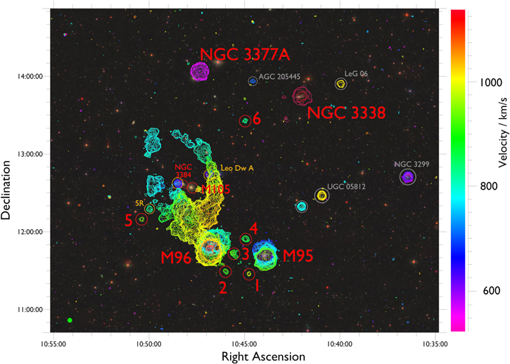
Figure 3. Renzogram of the whole survey region over the velocity range of the M96 subgroup. Each H i contour is at 3.5σ and colored according to velocity, overlaid on an RGB image from the SDSS. The Arecibo beam size (35 , 11.3 kpc) is shown as a filled green circle in the lower left corner. H i clouds are numbered, and selected major galaxies are labeled in red. Other objects used for a few comparisons but not examined in detail are highlighted in orange, while other known objects not used in this study (here shown for the sake of completeness) are highlighted in gray. The interactive version shows H i isosurfaces of constant S/N levels, as well as the galaxies with known optical redshift measurements in this region, found by an NED search. The user can pan (left button drag), rotate (middle button drag), and zoom (scroll wheel) around this region. Particular features can be toggled using the menu on the left, including the H i and bright and faint galaxies (i.e., members of the NGC and/or Messier catalogs or others)—note that the display of the menu is optimized for full-screen display, which can be enabled using the button at the lower right of the screen. Clicking individual galaxy labels gives the option of selecting a link to the SDSS DR16 Navigate tool centered on the coordinates of the object (hold "ctrl" while clicking to open in a new window).
Download figure:
Standard image High-resolution image Figure data file3.2. Other Wavelengths
The presence of the giant H i ring has attracted many searches for optical features of low surface brightness, including dedicated deep optical imaging in Schneider (1989), Ferguson & Sandage (1990), Michel-Dansac et al. (2010), and Watkins et al. (2014), the latter reaching a sensitivity of μB = 31.0 mag arcsec−2. In addition, Karachentsev & Karachentseva (2004) used reprocessed Palomar Sky Survey data to search for low surface brightness galaxies, while Müller et al. (2018) performed sensitivity enhancement on SDSS data to search for ultradiffuse galaxies (UDGs). We searched the catalogs from all of these papers. In addition, we stacked both the SDSS g-, r-, and i-band data and (separately) the Digitized Sky Survey blue and red images, searching the position of the clouds within the Arecibo beam area.
We found no hint of any optical counterpart for clouds 1, 2, 3, and 6. While there is a galaxy (LeG 46) 20'' from the H i coordinates of cloud 5, the SDSS optical redshift is >28,000 km s−1, and it is therefore unassociated. Only cloud 4 has a clear detection at optical wavelengths: the galaxy LeG 13 (AGC 202024). We regard the optical counterpart as being almost certainly associated with the H i emission even though there is no corroborating optical redshift measurement, as the optical and H i coordinates differ by just 13'' (with no other similar objects nearby). Furthermore, the optical component is sufficiently resolved that it appears more likely to be a group member than a more distant background object. There are no instances in the rest of the AGES sample of finding a single optical counterpart candidate so close to the H i coordinates in which, where available, the optical redshift determination did not closely match the H i measurement. The possibility of a coincidental alignment of the optical and H i components can therefore be neglected.
Although it is only marginally more massive than the other clouds, cloud 4 is also the only cloud in this sample detected by ALFALFA (Stierwalt et al. 2009; Haynes et al. 2018). The ALFALFA data (Stierwalt et al. 2009) gives a slightly lower H i mass (6.4 ×10⁶ M⊙) than the AGES estimate (9.0 ×10⁶ M⊙), and the estimated velocity widths from ALFALFA (W50 = 24 km s−1, W20 = 37 km s−1) are also slightly lower than the AGES values (W50 = 31 km s−1, W20 = 46 km s−1). This difference is unsurprising given the differing sensitivity levels. We hereafter only use the more sensitive AGES measurements, which have a high S/N level and a detection that is clear and unambiguous in the spectrum.
The ALFALFA SDSS catalog (Durbala et al. 2020) provides two estimates of the stellar mass for LeG 13 (i.e., cloud 4)—we use the mean value of 6.6 × 10⁶ M⊙; the individual values differ by a factor three. This gives an MH i /M* ratio of 1.4 (no star formation rate estimate is available in the catalog, as it is not detected in Wide-field Infrared Survey Explorer (WISE) band W4 and does not have a UV flux measurement in the NASA-Sloan Atlas, the criteria required for the star formation estimates of Durbala et al. 2020). Given this ratio and that the H i mass is only marginally higher than in the other clouds, it is not obvious why cloud 4 has an easily detectable optical counterpart but the others are, if perhaps not actually dark, then significantly fainter. However, we caution that LeG 13 is itself only detected at about 6σ in the SDSS. This implies that the MH i /M* ratio of the other detections need not be extraordinarily high for the optical counterpart to be undetectable, perhaps only of order a few (contrast this with the more massive H i detection of Józsa et al. 2022, which has a ratio in excess of 1000), though the deeper optical imaging of the studies cited above would likely have revealed such an object.
4. Analysis
There are two main possibilities for the nature of the clouds: transient tidal debris, and long-lived galaxies in which the H i resides in a dark matter halo and the line width indicates rotation. We follow the analysis presented in Taylor et al. (2016) for the clouds discovered in the Virgo Cluster.
4.1. Size of the Clouds
Cloud 3 is marginally resolved, with the 3.5σ contours spanning approximately two beams. This gives a diameter of ∼20 kpc. Although the other clouds are not resolved, the large size of this cloud and its similar mass tentatively suggest that the others are unlikely to be much smaller than the beam size.
At a typical mass of 5.0 × 10⁶ M⊙, a source filling the 11.3 kpc diameter beam would have a column density of 0.05 M⊙ pc−2 (6.3 × 1018 cm−2). Conversely, to have a column density of the more typical 6 M⊙ pc−2 found in dwarf galaxies (Leroy et al. 2008), the diameter would be around 1 kpc. Such a column density is technically possible, as the circular-average column density may be misleading: since even cloud 3 is only marginally resolved, it is possible that it is much smaller along one axis. But while a higher column density is consistent with observations, it is unlikely that this is actually the case. At densities comparable to dwarf galaxies we would expect to see star formation and therefore optical counterparts. The true size of most of the clouds is therefore likely of the order of a few kiloparsecs, especially given the size of cloud 3; supporting evidence of this can also be found in Section 4.4.
We can more confidently rule out that the clouds might be gravitationally self-bound by their H i mass alone. As with the Virgo clouds, this would require an unphysically high column density (≫100 M⊙ pc−2, a value that is unknown for H i, with a diameter of 0.1 kpc) even given the Leo clouds' lower velocity widths. We would certainly expect to see obvious optical counterparts at densities this high, though only cloud 4 has any direct association with an optically bright galaxy. Note that while cloud 4 does have the highest H i mass of the clouds, it is less than a factor two greater than their median H i mass.
4.2. Expansion Time
If the clouds are unstable debris, the line width can give an indication of their detectable lifetime. For the high velocity dispersion clouds in Virgo, we found that the lifetimes were so short as to make a tidal debris hypothesis unlikely. In contrast, the Leo clouds have substantially narrower line widths, which does not give such a stringent constraint on their evolution. For cloud 3, which is marginally resolved, to reach its 11 kpc radius at its presumed expansion velocity (W50/2 = 21 km s−1) would take 0.5 Gyr. Therefore, with similar expansion speeds and assuming sizes half that of cloud 3, the other clouds could have existed for ∼250 Myr.
Although obviously approximate, these estimates can be considered upper limits of the cloud survival times based on their line widths. We have assumed that the clouds began as point sources, which is unphysical—a more realistic initial size could only lead to shorter expansion times. Likewise, we assume that the clouds fill the beam, whereas most of them are probably somewhat smaller (but see Section 4.4 for an important caveat). More significantly, in some cases the W20 value, which is much larger than the W50 value, is a more accurate estimate of the true line width (see Section 4.7), and using this value for the expansion velocity would roughly halve the timescale estimates. Even so, the long lifetime estimates are at least consistent with the clouds being tidal debris, but we consider this further in Section 4.4.
4.3. Dynamical Masses
The optical counterpart of cloud 4, AGC 202024 (LeG 13), allows for different interpretations of the nature of the clouds. One possibility is that the clouds are tidal debris in different stages of evolution, with only cloud 4 as yet having undergone any significant star formation, or perhaps the only one in which star formation continues (see Román et al. 2021 for a discussion on fading tidal dwarfs). Another option is that most clouds are tidal debris but cloud 4 is an ordinary galaxy, and its close position and similar H i properties to the other clouds are purely coincidental. It is also possible that the clouds are in fact all primordial galaxies (e.g., satellites), with their H i embedded in dark matter halos. In this case cloud 4 would be significantly optically brighter than the others, though this does not necessarily mean that the other clouds are totally dark. In this interpretation, we can use their line widths to estimate their dynamical masses, i.e.,

For cloud 3 we may take the radius to be 11 kpc since it is marginally resolved. With a rotation speed vcirc of W50/2 = 21 km s−1 (note that though the line width is small, it does appear to show a velocity gradient—though we lack sufficient resolution to say whether this is the result of ordered motions), this gives Mdyn ≥ 1 × 10⁹ M⊙ (this is a lower limit, as we do not correct for inclination), giving a ratio Mdyn/MH i ≥ 140. This would be an extremely dark-matter-dominated object.
For the other clouds, assuming a radius of 5.5 kpc (half the beam size) and a typical line width 30 km s−1, dynamical masses would still exceed 3 × 10⁸ M⊙, with Mdyn/MH i ≳ 50. At the smallest plausible size of a radius of 0.5 kpc (see Section 4.1), Mdyn ≥ 3 × 10⁷ M⊙ and Mdyn/MH i ≳ 5. Despite their low line widths, the clouds are consistent with requiring a significant quantity of dark matter in order to be stable and long-lived.
4.4. Environment of the Clouds
4.4.1. Clouds 1–4
The proximity of the nearest galaxies is crucial to understanding the origin of the clouds. Clouds 1–4 are midway between the giant spiral galaxies M95 and M96, which have a projected separation of approximately 0 7, equivalent to 136 kpc. The clouds are also at similar velocities to the two spirals (M95 is at 779 km s−1, M96 is at 888 km s−1), as shown by the PV diagram in Figure 4. Cloud 1 is, however, somewhat deviant from the trend in PV space seen from clouds 1–4.

Figure 4. PV diagram of the M95–M96 region with a linear color stretch, highlighting clouds 1−4.
Download figure:
Standard image High-resolution imageIn Section 4.2 we calculated that the clouds could have survived for as long as 250 Myr even if in free expansion. To travel the approximate 70 kpc from the nearest spiral in 250 Myr would require a projected velocity of 270 km s−1. In comparison, the dispersion of the Leo I group as a whole is 175 km s−1 (Stierwalt et al. 2009), with the line-of-sight velocity differences of the clouds from M95/M96 ranging from 6 to 181 km s−1. However, 70 kpc is considered from the distances to the centers of the galaxies. A more realistic value, accounting for the apparent size of the H i disks, would be about 40 kpc, reducing the velocity to about 150 km s−1. Given that the survival timescales are approximate upper limits and that the true 3D velocity must necessarily be higher than the projected velocity estimate, it seems reasonable to say that the clouds are consistent with being tidal debris, albeit with velocities toward the higher end expected for objects in this environment.
Perhaps more problematic for this interpretation is that neither M96 nor M95 show much indication of a significant disturbance in their H i disks. M95 in particular shows no signs of abnormality—by the criteria established in Taylor et al. (2020), we would identify this galaxy as undisturbed. In contrast, M96 does show evidence of a warp (this is much easier to see in the online 3D tool than the renzogram or PV map), as well as being asymmetrical in its optical appearance, but not any larger extension that could be identified as a tail that would indicate gas removal.
One possibility is that the clouds in this region are the brightest peaks in a lower-density bridge of material connecting the two galaxies, as suggested for the M31–M33 clouds (Wolfe et al. 2013). If so, the large-scale H i feature expected in tidal encounters (Taylor et al. 2016, 2017) would exist but happen to be below our column density sensitivity. We investigate this in Figure 5 (see Figure 3 for a map of the whole survey region). The figure shows renzogram contours at the 3.5σ level from the standard AGES cube and also thinner contours at 4σ from the cube after additional Hanning smoothing (width 15 channels, equivalent to 40 km s−1 resolution) of the spectral axis—spectral smoothing has the advantage of increasing sensitivity without degrading spatial resolution. The smoothing reduces the rms to 0.3 mJy, about half that of the standard cube. Note that, due to the lower spectral resolution, the sensitivity to total mass present, i.e., column density, is degraded to NH I = 3.0 × 1017 cm−2 at 1σ—smoothing improves the sensitivity to the average mass present per unit velocity, which is the relevant factor when searching for diffuse emission.

Figure 5. Renzogram of the M95–M96 region. The thick contours are from the standard AGES cube at 3.5σ. The thin contours are from a cube with additional Hanning smoothing (width 15) at 4σ. The green circle in the upper right corner shows the AGES beam. An additional feature tentatively identified as cloud 7 is also shown.
Download figure:
Standard image High-resolution imageInterestingly, this extra smoothing does not alter the appearance of M96, M95, or cloud 1, but the other clouds do appear more extended. Cloud 2 shows a tentative connection to M96. Somewhat surprisingly, cloud 4 appears to be marginally resolved, spanning approximately two beams—given that it has an optical counterpart, we would expect it to have a higher column density than the other features and so be more compact, yet this is not the case. However, this is a further indication that our size estimates in Section 4.1 are unlikely to be wide of the mark. Cloud 3 becomes significantly more extended, spanning four beams (45 kpc) with a clear velocity gradient across the whole feature (the velocity difference between the most extreme contours where the cloud is visible is 67 km s−1), though it does not appear to directly connect with the disk of M96.
The extra Hanning smoothing also reveals a tentative additional detection here labeled as cloud 7. In the standard cube this is just visible but appears as an extension of cloud 2. Due to its small size (the contours do not even span a whole Arecibo beam) and low S/N (peak 5.4, integrated 6.25), we treat this detection with caution. If real, it would have an H i mass of 3.5 × 10⁶ M⊙, a W50 value of 52 km s−1, and a W20 value of 80 km s−1.
Despite the detection of extended features and a possible additional cloud, the extra processing does not reveal any large-scale bridge of material linking M95 and M96—at this sensitivity level, there is no evidence that the clouds are peaks in a larger structure. While cloud 2 does resemble some of the clouds discussed in Keenan et al. (2016; where features that appeared as discrete at a lower sensitivity were revealed as being connected to the disk of M33 at a higher sensitivity), the smoothing does not suggest that the disk itself is likely to be much larger than it appears in the standard cube. This does not rule out a tidal origin for the clouds, but it does not fit the general expectation of tidal stripping.
Of course, the elephant in the room is the Leo Ring—M96 is directly connected to the main body of the Ring, 7 and it is possible that M95 was also involved in the creation of this feature. Potentially M96 could be interacting with the other major galaxies in the Ring (e.g., M105, NGC 3384), as well as M95. It is interesting to note that clouds 2, 3, and 4 are close in velocity to the warp seen in the H i of M96—again, in PV space these clouds do resemble a bridge, but this is not seen in position–position (PP) space.
Finally, another scenario is that the clouds are not the result of a direct interaction between M95 and M96 but rather result from whatever process formed the Leo Ring. The appeal of this explanation is that the Leo Ring has a velocity width of ∼400 km s−1, making it much easier for the clouds to reach a large separation from their parent galaxies (see also Section 4.5). On the other hand, the kinematics of the clouds do not match the velocity gradient of the Ring at all, being at velocities approximately 150 km s−1 lower than the material in the nearest point on the Ring.
Though these caveats are important, overall the evidence would still seem to point toward a tidal interpretation for clouds 1–4. They lie midway between two galaxies, one of which shows signs of disturbances (albeit more weakly than we would expect), and at a distance consistent with the clouds being unstable debris. The lack of a large stream of H i is, in our view, a relatively minor difficulty in this case. Despite the increase in sensitivity from smoothing, it is still possible that such a stream exists but is below our detection threshold, with the clouds being significant density enhancements within it (as in Wolfe et al. 2013). In our Virgo simulations (Taylor et al. 2016, 2017), we found that clouds themselves detached from their parent galaxies were usually found near large, easily detectable H i tails that were directly connected to their parent galaxies. Such features are not seen here unless we count the Ring itself, but the cluster and group dynamics are markedly different. Simulations of low velocity dispersion groups could help address whether (and for how long) we should expect large streams to accompany detached clouds in these environments, and/or whether the detached clouds themselves are an expected result of tidal encounters.
4.5. Clouds 5 and 6
While it does appear distinct, cloud 5 is in close proximity to the Leo Ring. This region of the Ring is highly disorganized, and it is possible that this is an outlying cloud formed by the same processes that produced the rest of the large-scale H i emission in this region. To the north, a much larger and more massive cloud is also detached but appears to be part of the Ring. Whereas the northern feature clearly fits neatly into the ellipsoid structure of the rest of the H i, cloud 5 is not aligned with any other features. Moreover, the additional smoothing described for clouds 1–4 does not reveal any additional component to cloud 5, and its narrower line width suggests that it is—at least at present—truly detached from the Ring and not an outlying part of the larger object. Still, the most obvious explanation is that cloud 5 was produced along with the rest of the Ring, a process we will explore in a future work.
Cloud 6 is much more intriguing. While it is possible that it, too, was formed by the same mechanism that created the ring (e.g., the collisional origin proposed by Michel-Dansac et al. 2010), its distances and kinematics argue against this interpretation. It is 065 away from the nearest point on the Ring, about 125 kpc in projection, and does not align with any features in the Ring. The distance to M105, at the approximate center of the Ring, is about 11, 210 kpc. At the estimated evolution time of 250 Myr (Section 4.2), this would require a projected velocity of 820 km s−1. Almost all of this would have to be across the plane of the sky, since the velocity of the cloud falls well within the velocity of material of the Ring. In contrast, the Ring itself only spans about 400 km s−1. The kinematics of the cloud and the Ring thus do not match: it is very difficult to see what sort of process could produce a gigantic, coherent arc of material and also one single, compact cloud that was ejected at least at twice the velocity of everything else. While we cannot absolutely exclude a common origin of the Ring and cloud 6, there are other possible candidate parents for the cloud.
There are four other nearby H i–detected galaxies that suggest themselves as potential parents based on their angular separation from cloud 6. Two of these, UGC 05832 (a disturbed spiral) and CGCG 065–090 (an irregular), form a close pair, and we cannot fully distinguish the H i detection of the individual galaxies in this case. These are at least 047 away in projection (90 kpc) from the cloud, with a velocity separation of 360 km s−1. As discussed in the introduction, this velocity difference is much greater than the group velocity dispersion, making an association less likely. Near to this pair of galaxies is a third, much more massive spiral NGC 3338 (note that while the pair are not visible in Figure 3, as they are outside the velocity range shown, part of NGC 3338 is just visible). This is rather farther away at 077 (147 kpc) and even more separated in velocity (440 km s−1) from the cloud. While the spiral/irregular pair do show disturbances in their optical morphology, none of these three galaxies show significantly extended H i emission: we can easily distinguish the H i in the pair from the giant spiral, and there is no hint of any extension toward cloud 6.
In addition, NED gives a mean redshift-independent distance estimate to NGC 3338 of 22.6 Mpc, twice the distance to the M96 subgroup. Likewise, the fact that all of the clouds are found within a velocity range of 100 km s−1 while UGC 05832 and CGC 065–090 are found at a difference of 360 km s−1 argues against their association with any of the clouds. Again, given the low velocity dispersion of the Leo Group, it seems much more probable that all the clouds are found at this much lower distance and are unrelated to any of the background galaxies.
The fourth candidate is the spiral NGC 3377A, rather uniform in morphology, which is 086 (164 kpc) away in projection and separated in velocity by 287 km s−1 from the cloud. As with the other candidates, this galaxy also shows no hint of any H i extension, and its velocity separation is quite high compared to the dispersion of the M96 subgroup.
Frustratingly, none of these candidates can be definitively assigned or eliminated as the parent of cloud 6. The H i masses of all four candidates (Stierwalt et al. 2009) range from two to four orders of magnitude greater than the clouds, implying that we should easily be able to detect any disturbance in the parent galaxy sufficient to account for the clouds. The low mass of the clouds means that estimating the H i deficiencies of the candidate parent galaxies would be useless since they would only constitute a small fraction of any missing gas (see Taylor et al. 2017 for a discussion on the well-known, more massive example of VIRGOHI21 and its parent galaxy NGC 4254).
4.6. Comparisons with Other Clouds
In Taylor et al. (2016) we presented a table of isolated dark clouds with possible primordial origins. Very few clouds are known that are similar to the Leo clouds. We briefly review those with notably similar features below. These were selected on the basis of being clearly detached from their parent galaxies (which are usually difficult to identify) and having no large-scale extended H i emission (such as tails) visible in their vicinity.
4.6.1. GBT1355+5439
Discovered in Mihos et al. (2012) and with follow-up observations described in Oosterloo et al. (2013), this cloud is located close to M101 in projection. Due to its low systemic velocity (210 km s−1), the distance is highly ambiguous. If this object is in the Local Group, then Oosterloo et al. (2013) propose that it could be a dark matter minihalo, with a size of about 1 kpc and MH i ∼1 × 10⁵ M⊙. At the distance of M101, it would be 150 kpc from M101 with an H i mass just a bit larger than the Leo clouds at 1 × 10⁷ M⊙. The W20 is given in Mihos et al. (2012) as 41 km s−1; W50 is not reported. Oosterloo et al. (2013) concluded that there is no clear explanation for the object, with all of the proposed interpretations (galactic minihalo, dark galaxy, tidal debris) having advantages and disadvantages.
4.6.2. GEMS_N3783_2
Discovered in Kilborn et al. (2006) in a survey of the NGC 3783 group, this cloud is considerably more massive than the Leo clouds at 3.8 × 10⁸ M⊙. The W50 value is 106 km s−1, and the W20 value is 116 km s−1. Although the nearest spiral does show an extended, distorted H i disk that might indicate an interaction, it is 450 kpc away from the H i cloud and does not show any long H i tails. Kilborn et al. (2006) do not rule out a dark galaxy interpretation, but they consider a tidal origin more probable.
4.6.3. NGC 1395 Clouds
Wong et al. (2021) discovered two clouds (C1 and C2) in the vicinity of NGC 1395, of mass (2–3) × 108 M⊙—again considerably more massive than the Leo clouds. These clouds appear to be of similar velocity width to the Leo clouds, with W50 measured at 17–41 km s−1 from ATCA and Parkes, respectively (W20 is not reported—from the figures, W20 may be substantially higher but affected by noise). Unfortunately, one cloud is projected in front of the elliptical galaxy NGC 1403, hampering the identification of any optical counterparts (NGC 1403 itself almost certainly has no association with the cloud; it is at a systemic velocity more than 2000 km s−1 higher than the H i detection). The clouds range from 240 to 360 kpc in projected distance from NGC 1395. In marked contrast to the Leo clouds, Wong et al. (2021) note that the line width and size of these clouds are consistent with being gravitationally self-bound by the mass of the H i alone. Their favored hypothesis is that the clouds could be optically dim or dark tidal dwarf galaxies, though the lack of any observed tidal tails in the region is arguably problematic for this interpretation.
4.6.4. SECCO 1
SECCO 1, also known as AGC 226067, is discussed in Adams et al. (2015), Bellazzini et al. (2018), and Calura et al. (2020). The object is an optically faint (but not dark) H i cloud in the direction of the Virgo Cluster. Candidate parent galaxies are at least 250 kpc away in projection, and the stellar component appears to lack an old population. Its H i mass is a bit larger than the Leo clouds at 1.5 × 10⁷ M⊙ (at the Virgo Cluster distance), as is its W50 line width at 54 km s−1. Simulations in Bellazzini et al. (2018) show that a low line width cloud could survive for over 1 Gyr moving through the intracluster medium, certainly long enough for the cloud to have reached its separation from its candidate parent galaxies. What remains unclear is why, if there is really no old stellar population, the star formation should apparently have begun only very recently despite no obvious source of perturbation.
4.7. The Baryonic Tully–Fisher Relation
One of the most intriguing features of the AGES Virgo clouds is their offset from the baryonic Tully–Fisher relation (BTFR). Most normal galaxies appear to show a tight correlation between their rotation velocity and baryonic mass (McGaugh et al. 2000). While some UDGs have been found to have velocity widths well below the expectations from the BTFR, given their baryonic mass (Mancera Piña et al. 2020 8 ), the AGES Virgo clouds of high line widths show the opposite behavior. In Figure 6 we compare the AGES Virgo and Leo clouds on the BTFR, along with a selection of other optically dark clouds from other surveys. We also include other features found in Leo: the tentative feature dubbed cloud 7 (see Section 4.4), the faint galaxy Leo Dw A (Figure 3, Schneider 1989), the cloud adjacent to NGC 3384 (Figure 3; note that the measurements are uncertain owing to the close proximity of material from the Ring), and a "cloud" labeled 5R (again see Figure 3), which is likely part of the Ring itself.

Figure 6. BTFR for normal galaxies (black circles, from the AGES Virgo background fields) and a selection of optically dark H i clouds, using the W50 (left) and W20 (right) estimates for the line width. The line widths are corrected for inclination for the galaxies but not the H i clouds. The baryonic mass for the clouds is computed using their H i mass multiplied by a factor 1.36 to account for the presence of helium. The dashed line is the best fit to the optically bright galaxies. Our main sample of Leo clouds are shown with red squares, while additional objects in Leo are shown as open red squares (highlighted with orange circles in Figure 3; cloud 7 is shown in Figure 5). Clouds from the Virgo surveys of AGES are shown with open blue circles, while other clouds in the Virgo Cluster are shown as labeled open blue squares. Other clouds in green are described in Section 4.6. The solid line in the left panel shows the completeness line for an integrated S/N of 6.5.
Download figure:
Standard image High-resolution imageThe results vary depending on whether we use the W50 or W20 estimators for the line width. Before discussing this in relation to the clouds, it is important to note that this is also true for normal galaxies, with three optically bright galaxies having apparently anomalously low circular velocities when using W50 but normal values (i.e., lying well within the general scatter) when using W20. This is not because they are similar to the Mancera Piña et al. (2020) objects, but only because of the profile shape: a high S/N but narrow spike can lead to an erroneously low value for W50, even when the W20 estimator is still itself at a high S/N level. We consider the W20 estimate to be generally more reliable for the Virgo clouds, and the deviation toward high velocities is seen even using W50 for some of them. It is important to note that neither W50 nor W20 is an infallible measure of the true width of the line. While W20 may give overestimates due to being measured at a lower S/N level, W50 can give underestimates despite being measured at a higher S/N level (possible improvements to measuring the velocity width are described in Yu et al. 2021, 2022).
Some of the Leo clouds appear to follow the BTFR for bright galaxies. Ostensibly, there is no particular reason to expect tidal debris to follow the BTFR—nonrotating, unbound debris (regardless of its formation mechanism, tidal or otherwise) has no constraints to follow the same relation as for rotating, stable galaxies. In the case of the Leo clouds, most seem likely to have formed as a result of interactions, based on their proximity to galaxies and/or the Leo Ring, with the notable exception of cloud 6. Yet most of the clouds in our Leo sample do seem to follow (or are found close to) the BTFR for normal galaxies—including features that seem to be part of the Ring (the single exception is the tentative detection of cloud 7, which we discuss further below). An important caveat is that, using W50, most of the clouds are found at higher velocity widths than expected, with only cloud 5 at lower velocities (though clouds 4 and 5R are very close)—if the clouds were really following the relation, we might have expected about half to have higher and half to have lower widths than the general relation.
There is no obvious reason why the clouds should follow (or be close to) the BTFR for bright galaxies, as it cannot be a selection effect. Given the typical maximum column density of H i of ∼10 M⊙ pc−2 (Leroy et al. 2008) and the beam size, we could expect to detect up to 109 M⊙ of H i within the Arecibo beam at the 11.1 Mpc of the group—about two orders of magnitude greater than the BTFR implies for clouds of these line widths. Indeed, as discussed, dark clouds are known elsewhere that are considerably more massive than the Leo clouds and that do show a strong deviation from the BTFR.
Conversely, we can also consider how large the line widths of the clouds would be for them to become undetectable if their mass were kept constant. Although the clouds have narrow line widths, they are reasonably bright. By the prescription of Saintonge (2007) we should be complete to sources of these typical masses (equivalently, ∼ 0.2 Jy km s−1 flux) for velocity widths of up to 130 km s−1, far wider than their actual values. In short, there is nothing prohibiting the existence of much more massive clouds given their observed ∼30 km s−1 widths, nor any reason they could not be detected at much higher line widths for the same total flux: they could be detected over a much larger part of the BTFR parameter space than the region in which they are actually found.
Examining the W20 estimator complicates the situation. Using W50, most Leo clouds are found at somewhat higher velocities than the fit for optically bright galaxies, even if only slightly. For W20, most lie closer to the fit, but there are some stronger deviations as well. With W50, of our Leo objects, only cloud 7 shows an appreciable deviation from the standard BTFR, whereas with W20, a similar deviation is also seen for cloud 1 and possibly the cloud adjacent to NGC 3384. The faint nature of cloud 7 implies a need for observations of high sensitivity and especially of higher spatial resolution than AGES to determine whether this is really a discrete object or only part of cloud 2, and similarly accurate measurements of the NGC 3384 cloud are confused by intervening material from the ring—it is likely that the W20 measurement is an overestimate in this case. Intriguingly, the W20 measurement of cloud 1 appears to be accurate—indeed, if anything, it seems more likely that the W50 measurement is an underestimate. We note that, unlike the other clouds, its spectral profile is clearly asymmetric (Figure 1), suggesting that it might have multiple components, and reinforcing the need for higher-resolution observations. Based on their proximity to other galaxies and H i structures, all of the Leo objects with excessively high W20 values are likely tidal in origin.
An important caveat is that the results discussed above are sensitive to the best-fit line used for the BTFR, which in Figure 6 is heavily dominated by optically bright galaxies that are more than two orders of magnitude brighter than the optically dark clouds. For this figure we used the same basic methodology as in Taylor et al. (2013): the baryonic mass is the combination of the measured MH i (with an assumed correction for helium) plus the stellar mass, with the line width corrected only for inclination. This approach has the advantage of simplicity and relies entirely on our own measurements. A more sophisticated approach necessitates greater complexity in correcting the measurements but allows us to compare our results with the gas-dominated, lower-mass sample presented in McGaugh (2012). This should provide a more robust comparison with the Leo clouds, in particular a quantitative assessment of how well they agree or deviate from the BTFR for normal galaxies given the general scatter. Importantly, McGaugh (2012) used resolved rotation curves to estimate the circular velocity, which gives much more accurate results than line widths. Note that the corrections applied to our own data are extensive and fully described in Appendix. The result is shown in Figure 7.

Figure 7. BTFR using more sophisticated corrections for velocity width (derived for our sample from W20) and stellar mass, following the prescriptions of McGaugh (2012) and Springob et al. (2005)—for full details see Appendix. The color scheme is as for Figure 6, except that the open circles show the sample of McGaugh (2012, his Table 1). The black solid line shows the best-fit relation according to McGaugh (2012), with the dashed and dotted lines showing the 1σ (0.24 dex in mass) and 2σ scatter, respectively, again according to McGaugh (2012). Clouds from non-AGES samples are not included, as we lack the data needed to make the appropriate corrections to velocity width, which is corrected for inclination, spectral resolution, and cosmological expansion.
Download figure:
Standard image High-resolution imageFigure 7 supports the basic result of the right panel of Figure 6. Clouds 1 and 7 and the NGC 3384 feature clearly deviate from the BTFR in the sense of having an unexpectedly high velocity width, while cloud 5 may have a width somewhat lower than expectations. Clouds 2, 4, 6, as well as 5R and Leo Dw A, all lie well within the general scatter. Cloud 3 is a marginal case, having a velocity width slightly exceeding the 2σ scatter. Overall, the main result appears robust: some clouds do deviate from the BTFR, but others do not. We note that there is a significant caveat in that the exact form of the BTFR depends strongly on the corrections used, especially for the stellar mass, with McGaugh (2005, 2012) describing how the slope—the exponent in the power-law fit—can vary from 3 to 4; readers are strongly encouraged to consult Appendix for details.
While these deviations from the BTFR might seem to indicate that these clouds do indeed have a nongalactic nature (i.e., they are transient and unstable), several difficulties arise. This does not explain why the other objects stubbornly remain within the observed scatter of the BTFR, including cloud 4 and arguably cloud 3, which are both close in projection to clouds 1 and 2 (with significant caveats: cloud 3's extended nature may mean that its velocity width has been underestimated, while cloud 4 has an optical counterpart and so may be an ordinary galaxy). Moreover, the similarly excessive velocity widths of the Virgo clouds have proved difficult to explain: in Taylor et al. (2016), we found that it was very difficult to reproduce the high velocity widths of the Virgo clouds if they were produced as tidal debris, 9 whereas if they were faint or dark galaxies, their deviation from the BTFR could be easily explained and was robust to tidal interactions with other galaxies. However, as discussed, the dynamics of tidal encounters in a cluster will be significantly different than in a group environment, again indicating a strong need to simulate a more Leo-like region before any firm conclusions can be drawn.
Of the non-AGES clouds, even more caution is needed since the values for W50 and W20 are not reported homogeneously (they are shown in Figure 6 but not Figure 7, as we lack the data for corrections necessary to estimate their velocity widths). Both of the Wong et al. (2021) clouds appear to have lower-than-expected velocity widths given their gas mass, even using the line widths without any additional corrections: Wong et al. (2021) note that while the clouds do appear to be rotating, W50 likely overestimates the rotation velocity with a significant component of the line width originating from velocity dispersion. The other two clouds (GBT 1355+5439 and GEMS_N3783_2), though differing in mass by almost two orders of magnitude, both lie on the same BTFR as for normal galaxies. The amount of intrinsic scatter on the BTFR is controversial, with Mancera Piña et al. (2020) arguing that some galaxies are strongly deviant (see also Mancera Piña et al. 2022), whereas Lelli et al. (2016) say that the intrinsic scatter is below Standard Model expectations, and McGaugh (2012) find that there is no scatter unexplained by observational errors. If the latter is correct, then it seems remarkable that this is even true for some objects that are likely debris, where the usual dynamical relations should not apply. Paradoxically, it seems that some objects for which the evidence generally indicates a tidal origin (e.g., clouds 1–5 in Leo) actually lie on the standard BTFR, while some for which the evidence is—arguably—against a tidal origin (e.g., the AGES Virgo clouds, the Mancera Piña et al. 2020 UDGs) clearly deviate from it. This is exactly opposite to what we might expect.
5. Summary and Discussion
We reported the discovery of at least five optically undetected H i clouds in the M96 subgroup. One of the objects (cloud 5) is close to the giant Leo Ring and most likely part of that structure—we leave analysis of this to a future work. Three of the optically undetected H i clouds (as well as an additional more tentative detection not included in our main sample) lie between M96 and M95, suggesting a tidal origin. In PV space these clouds appear to be part of a bridge connecting the two spiral galaxies, but in PP space this structure is not seen. No elongated structures directly attached to M95 are visible, though M96 is connected to the Ring. Very near to these three clouds, and at a similar velocity, the dwarf galaxy LeG 13 (cloud 4 in our catalog) is detected with similar H i properties to the dark clouds but with a clear optical counterpart. Elsewhere in the group, another object (cloud 6) is seen with no apparent association with the Ring or any of the galaxies present. None of its nearest H i–detected neighbors show any signs of disturbances in their gas disks. With the nearby galaxies having H i masses two to four orders of magnitude greater than the clouds, which are themselves readily detected, even a small perturbation to their H i ought to be easily detectable with AGES—and their distances are anyway well outside the Leo Group. This makes the parent galaxy of cloud 6 extremely challenging to identify.
All of the clouds (including LeG 13) possess comparable H i masses and velocity widths, but in other aspects the clouds are dissimilar. While clouds 1–4 are all between M95 and M96, cloud 1 is offset in velocity from the others and has a higher velocity width. Cloud 2 may be connected to the disk of M96, while cloud 3 appears significantly extended when spectral smoothing is applied. Only cloud 4, LeG 13, shows an optical counterpart. Cloud 5 is near the Leo Ring, while cloud 6 is isolated.
Given this, it seems probable that the clouds formed from a variety of mechanisms, though a full exploration of this will require detailed numerical simulations. Overall, clouds 1–4 seem most likely to be tidal, but it is not at all obvious why cloud 4 alone is optically bright while its neighbors are undetected (it is tempting to suggest that since it has the highest H i mass it might have the highest column density, but its mass is only marginally greater than the others, and it shows some hints of being more extended as well). Cloud 6 is least likely to be tidal given its separation from its nearest galaxies, but the low line width of all clouds would allow them to survive travel across distances exceeding 100 kpc at velocities compatible with the group velocity dispersion. The main difficulty for the tidal debris interpretation is the lack of any elongated tails found around any of the galaxies in this region, the Leo Ring itself notwithstanding. If the clouds were produced by the same process that created the Ring, then they provide additional constraints for any future modeling efforts—in particular, it is not obvious how cloud 6 could be explained by a simple galaxy–galaxy collision model.
A further oddity for the tidal debris scenario is that most clouds seem to obey the BTFR seen for normal, stable galaxies. This is unexpected, as the clouds are bright enough that they could be detected at much higher line widths (with the caveat that they would have shorter detectable lifetimes) and large enough that they could have much higher gas densities before star formation would be expected. In essence, both their baryonic masses and velocity widths are not constrained by selection effects to obey the BTFR, but this is where the clouds are found nonetheless.
Ironically, it may be easier to explain the clouds with the excessive velocity widths than those that have the same widths as ordinary galaxies. Unlike the cases of the Virgo clouds, which remain poorly explained as tidal debris, most of the Leo clouds are relatively close to major galaxies. This means that they could indeed be unstable, transient features, as they would not have to survive for very long to reach their current separation from their parents. Cloud 6 is problematic in this regard owing to its isolation, but even here its line width is sufficiently low to allow for a slow dispersal.
Applying heavy spectral smoothing to the data revealed that some of the clouds are more spatially extended than in the standard cube, but we did not find any evidence that they are connected to each other—there does not appear to be any large-scale bridge connecting them, even for those clouds that are close in projection to each other. Although cloud 1 shows evidence of multiple kinematic components, spectral smoothing did not show that this cloud had any significant extensions. While we cannot absolutely rule out that the clouds might be part of a larger structure, in which case their measurements regarding the BTFR might have to be revised, we see no evidence for this in the data.
To summarize, there are a variety of possible explanations of the clouds, none of which can be definitively ruled out, but none are entirely satisfying either:
- 1.All the clouds are tidal debris: some appear too isolated for this, and none of the nearest galaxies show the expected long H i extensions.
- 2.All the clouds are galactic in nature, though some are optically dark or very dim: there is no obvious reason why one cloud should be optically much brighter than the rest.
- 3.Cloud 4, which alone has an optical counterpart, is a galaxy, while the rest are tidal debris: it seems an unlikely coincidence that cloud 4 should have such a qualitatively different nature from three other clouds in its vicinity with otherwise very similar quantitative H i properties.
- 4.If the clouds are tidal debris, some may have arisen in an interaction between M95 and M96 while some were produced by whatever process gave rise to the Leo Ring: the kinematics of the clouds do not match the velocity gradient of the Ring, and though M96 does show a warp in its H i disk, neither it nor M95 shows any larger-scale H i emission predicted in numerical simulations of the formation of tidal debris.
In short, the clouds are consistent with both tidal and galactic interpretations, and neither scenario can be definitively ruled out. We are currently examining a variety of formation scenarios for the Leo Ring using numerical simulations, which may eventually shed light on these smaller but intriguing clouds.
We are grateful to the anonymous referee, whose helpful suggestions improved the contents of this manuscript.
This work was supported by the Czech Ministry of Education, Youth and Sports from the large lnfrastructures for Research, Experimental Development and Innovations project LM 2015067; the Czech Science Foundation grant CSF 19-18647S; and the institutional project RVO 67985815.
This work is based on observations collected at Arecibo Observatory. The Arecibo Observatory is operated by SRI International under a cooperative agreement with the National Science Foundation (AST-1100968) and in alliance with Ana G. Méndez-Universidad Metropolitana and the Universities Space Research Association.
The SOFIA Science Center is operated by the Universities Space Research Association under NASA contract NNA17BF53C.
This research has made use of the NASA/IPAC Extragalactic Database (NED), which is operated by the Jet Propulsion Laboratory, California Institute of Technology, under contract with the National Aeronautics and Space Administration.
This work has made use of the SDSS. Funding for the SDSS and SDSS-II has been provided by the Alfred P. Sloan Foundation, the Participating Institutions, the National Science Foundation, the U.S. Department of Energy, the National Aeronautics and Space Administration, the Japanese Monbukagakusho, the Max Planck Society, and the Higher Education Funding Council for England. The SDSS website is http://www.sdss.org/.
The SDSS is managed by the Astrophysical Research Consortium for the Participating Institutions. The Participating Institutions are the American Museum of Natural History, Astrophysical Institute Potsdam, University of Basel, University of Cambridge, Case Western Reserve University, University of Chicago, Drexel University, Fermilab, the Institute for Advanced Study, the Japan Participation Group, Johns Hopkins University, the Joint Institute for Nuclear Astrophysics, the Kavli Institute for Particle Astrophysics and Cosmology, the Korean Scientist Group, the Chinese Academy of Sciences (LAMOST), Los Alamos National Laboratory, the Max-Planck-Institute for Astronomy (MPIA), the Max-Planck-Institute for Astrophysics (MPA), New Mexico State University, Ohio State University, University of Pittsburgh, University of Portsmouth, Princeton University, the United States Naval Observatory, and the University of Washington.
This work has made use of the Digitized Sky Survey. The Digitized Sky Survey was produced at the Space Telescope Science Institute under U.S. Government grant NAG W-2166. The images of these surveys are based on photographic data obtained using the Oschin Schmidt Telescope on Palomar Mountain and the UK Schmidt Telescope. The plates were processed into the present compressed digital form with the permission of these institutions.
Appendix A: Constructing the Baryonic Tully–Fisher Relation
In this paper we have shown three different version of the BTFR. In Figure 6 we use entirely our own data measurements, of both the AGES H i data and the optical photometry from SDSS data, using either W50 or W20 to estimate rotation width (the two panels are otherwise identical). In Figure 7 we attempt to match our data to those described by McGaugh (2012), which requires significant extra corrections. It is a legitimate question as to which best fit to the data is the best best fit, as this can affect whether the optically dark clouds really do match the relation obtained from optically bright galaxies or not. We therefore describe the procedure for Figure 7 here in full.
A.1. Distances
In all previous AGES papers we generally estimate the distance by assuming that galaxies are in pure Hubble flow with H0 = 71 km s−1 Mpc−1. We use the measured heliocentric velocity to obtain distance via d = vhel/H0. However, Durbala et al. (2020), who are concerned with accurate measurements for the BTFR, recommend using the estimation of Haynes et al. (2018): d = vCMB/H0 with H0 = 70 km s−1 Mpc−1.
We convert our measured vhel into vCMB using the NED velocity correction calculator. Converting R.A. and decl. to galactic longitude l and latitude b,

where, from Fixsen et al. (1996), vapex = 371 km s−1, lapex = 26414, and bapex = +4826.
We use this distance estimation for all galaxies with vhel > 3000 km s−1, i.e., beyond the Virgo Cluster (Haynes et al. 2018 use this only for galaxies with vhel > 6000 km s−1, with those at lower velocities having distance computed via a more complicated flow model). For galaxies below this redshift, our sample consists entirely of objects either in the Virgo Cluster or in the Leo Group, for which redshift-independent distance estimates are available. In Virgo, following Taylor et al. (2012), galaxies are assigned to distances of either 17, 23, or 32 Mpc depending on their spatial position, while in Leo, as described here, we assume a distance of 11.1 Mpc for all objects.
A.2. Inclination Angles
In Taylor et al. (2013) we used our own estimates of the inclination angle when correcting the line widths, and we use these values here in Figure 6. However, to ensure consistency, for Figure 7 we use the values provided in the SDSS by the "expAB_r" parameter as recommended by Durbala et al. (2020). We use this for both corrections to the velocity width and internal extinction, described below.
A.3. Atomic Mass
The total mass of H i is computed as in the main text via the equation

where SH i is the total H i flux and d is the distance in Mpc as described above. For Figure 7, correction for helium to get the mass of atomic gas is done by a simple multiplicative factor, Mgas = 1.33MH i following McGaugh (2012), while for Figure 6 we use a factor 1.36 for consistency with Taylor et al. (2013).
A.4. Stellar and Baryonic Mass
Stellar masses are computed using our own measurements of g- and i-band optical photometry from the SDSS. We use the apparent magnitudes mg,i given in Taylor et al. (2012). We correct these for galactic extinction to give
where the attenuation Ag,i is obtained from Schlafly & Finkbeiner (2011). Note that Durbala et al. (2020) favor the galactic extinction model of Schlegel et al. (1998); however, toward Virgo the choice makes little difference, as extinction here is anyway very low.
The extinction-corrected magnitudes are then converted to absolute magnitudes via the standard equation:

where d is the distance in parsecs. For Figure 6, following Taylor et al. (2013), no additional correction for internal extinction is made. For Figure 7 we correct for internal extinction using the method described in Durbala et al. (2020). First, we generate a correction factor γ that is zero if ME > 17.0; otherwise,


This is converted to the attenuation A:
where b/a is the "expAB_r" parameter obtained above. We then get our final values for the absolute magnitudes via
To convert to stellar mass, we require the i-band luminosity in solar units, which is obtained from

where Mi,⊙ is the absolute magnitude of the Sun at i band; following Durbala et al. (2020), we use 4.58, whereas in our earlier papers (i.e., Figure 6) we have used 4.48. We can now convert to stellar mass, again following Durbala et al. (2020):

While Durbala et al. (2020) rely primarily on g- and i-band photometry as we do, they also give prescriptions to convert to stellar masses based on WISE IR photometry. They give two different methods to estimate the stellar mass in this way. We have found that their "McGaugh" formulation gives a somewhat better agreement with the BTFR of McGaugh (2012), and therefore we convert our stellar masses to this approximation. Durbala et al. (2020) do not give a direct conversion between the stellar mass obtained above (the "Taylor" method in their nomenclature) and the "McGaugh" method; however, they provide a conversion between the "Taylor" stellar masses to the estimates of the GALEX-SDSS-WISE Legacy Catalog 2:

which in turn can be converted to the final stellar masses we use here,

Converting to linear units, the baryonic mass is then given simply by Mbary = Mgas + M*,McGaugh.
A.5. Line Widths
For Figure 6 line widths are converted to circular rotation simply by taking half of the inclination-corrected value:

For Figure 7 we employ additional corrections. Based on the McGaugh (2012) recommendation when using line width data, we only use the W20. We correct for finite spectral resolution following Springob et al. (2005). First, we calculate the S/N as S/N = (Fluxpeak − rms)/rms (note that the usual AGES peak S/N values are simply (Fluxpeak/rms)). We then compute a correction factor λ based on S/N and the velocity resolution vres (10 km s−1 for AGES):


This then lets us calculate the velocity width correction factor:

which we subtract linearly from the velocity width W50 or W20. We also correct for cosmological broadening, giving a final corrected velocity width of

This is then converted to a rotation velocity as above:
McGaugh (2012) fit the BTFR using resolved rotation curves but also provided an empirical correction factor to convert line width measurements to more accurate rotation velocities. This arises because line widths tend to represent the peak rotation velocity, which may be slightly higher than the flat part of the rotation curve. If Mgas > M*, no additional correction is applied. If Mgas < M*,
This is the final value for the velocity width used in Figure 7. While Springob et al. (2005) discuss possible additional corrections for turbulence, we have not applied this. Their favored correction of linearly subtracting 6.5 km s−1 is not appropriate for low line width objects, as this can cause very large shifts and thus is strongly dependent on minor errors (discussed below). In addition, the clouds that form the focus of the present work are conceivably dominated by turbulent motions, so trying to correct for this would be a strange choice—to have a fair comparison, it is far simpler not to correct for turbulence in either the galaxies or the clouds.
A.6. Sample Selection and Outliers
For Figure 6 we place only minimal restrictions on the sample: i > 45° and H i def < 0.6. The inclination cut is to avoid large errors in the velocity width due to small errors in the inclination measurement. The deficiency cut is because, as we discuss in Taylor et al. (2013), at high deficiencies we find galaxies with very low line widths even using the W20 line width. The reason for this is likely astrophysical, with the galaxies so stripped of gas that their remaining H i no longer fully probes their rotation curve. Since our interest here is in comparing the Leo clouds to the BTFR of normal galaxies, we exclude these unusual outliers from the plots.
For Figure 7 the emphasis is on accurately reproducing the BTFR of McGaugh (2012), and we impose an additional cut: peak S/N > 10.0. Equivalently this means that the S/N level at the flux level of the W20 measurement is 2σ, which ensures a minimal inaccuracy due to noise. This cut is crucial. Without it, there is a very much larger scatter than in the figure shown here. That there is anyway a larger scatter in the line width data than the McGaugh (2012) resolved rotation curve data is, as he discusses, unsurprising, and that most of the AGES galaxies lie within 2σ scatter of this relation is probably about as good as we can expect.
The peak 10σ cut is somewhat arbitrary, but as a selection criterion it is broadly consistent with the Leo clouds we examine here. By gradually reducing this cut, we find that we do not see significantly more or stronger outliers until we reach 6σ. All of the Leo clouds exceed 9σ. The Virgo clouds are a little fainter. The faintest is at 5.2σ, a level at which significantly more scatter is seen. However, the next faintest is at 6.5σ, above the threshold where we see additional outliers, and the rest exceed 7σ. Therefore, the choice of S/N cut for the plot does not greatly influence our comparison of the clouds with regard to the BTFR established for optically detected galaxies.
However, a few more significant outliers remain apparent in our normal galaxy sample. The two galaxies with surprisingly low velocity widths (AGESVC1 251 and 252) may be astrophysically interesting, but they are both faint sources with low measured line widths, and any errors in the inclination angle here may be significant. Two other galaxies (AGESVC1 230 and 288) have excessively high velocity widths. In both cases, examination of the spectra reveals peaks in the noise that just exceed the flux at 20% of the peak value, skewing the W20 estimate. When we correct for this, both galaxies actually lie within the 2σ scatter: if we apply the additional cleaning procedures (fitting a second-order polynomial to the whole data set) described in Section 2.1, the noise peaks are pushed below the 20% level and the measured width values are substantially reduced. This procedure was not used in the original published VC1 and VC2 data, as it was not thought necessary; it was implemented later as a way of addressing much more egregious problems due to changes in the data reduction software. In a future AGES data release we may consider remeasuring the parameters using homogenous data processing, but this is beyond the scope of the current work, and it would be unfair to retroactively remove selected outliers based on their deviation from the BTFR when this is the very thing we are trying to examine. Note that the optically dark clouds in Virgo also all have follow-up observations.
A.7. Comparison of the Different BTFRs
The different procedures adopted for the BTFR plots here cause substantial changes in slopes; exactly as discussed in McGaugh (2005, 2012), this changes the slope (the logarithm of the exponent) from 3 to 4. At Vcirc = 100 km s−1, given that this also changes the normalization, this is equivalent to a baryonic mass change of about 0.5 dex. McGaugh (2005, 2012) chooses the fit that gives a slope of 4, arguing that since this also gives the lowest scatter, this is more likely to be the correct value. Given the many different choices available when correcting the various aspects of the plot, we refrain from commenting on which is preferable; our intention here is to compare the clouds with established BTFRs rather than advocate for any particular methodology. In any case, the basic result that some clouds clearly deviate from the BTFR while some are within the general scatter appears to be robust.
The systematic effects in fitting the BTFR are the dominant source of error. For this reason we avoid showing error bars in the plots, as the formal measurement errors are misleadingly small. In the case of the Leo clouds the W20 errors are 5–15 km s−1, allowing for a maximum change in width of 0.1 dex (but note that we account for spectral smoothing above, and see the discussion below). The error in the measured H i flux is typically around 20%, allowing for a shift in mass of about 0.07 dex. Such shifts could in principle combine to move the clouds farther from the McGaugh (2012) relation, but it seems an unlikely coincidence that five features have been found that all lie within the observed scatter. Still, the only way to be certain would be deep interferometric follow-up.
Finally, another concern is whether the comparison of line widths from demonstrably rotating galaxies and the motions in clouds of unknown nature is physically meaningful. For the sake of homogeneity we have applied the same correction for rotation (i.e., halving the line width) for the clouds as for the galaxies, though we cannot correct their measurements for inclination. Therefore, if they are rotating systems, their velocities plotted here are lower limits, meaning that they might actually be outliers from the BTFR after all. However, any rotating system that deviates from the BTFR in this way would seem to be interesting almost by definition. Conversely, there is no particular reason to expect turbulence-dominated clouds to follow the usual BTFR. On this basis, we argue that the comparison is an interesting one regardless of the nature of the kinematics of the different objects.
Footnotes
- 7
The impression one gets from inspecting the data is that the H i of M96 is superimposed on that from the Ring. This is somewhat subjective, but clearly there is nothing like the classical tail and countertail structure predicted in most tidal encounters (Toomre & Toomre 1972).
- 8
- 9
Essentially, the higher the line width, the faster the dispersion and so the faster the clouds reach an undetectably low S/N—the more excessive the velocity widths, the shorter the lifetime of any such objects. See Taylor et al. (2017) for a full discussion.