


Abstract
Analyzing time-resolved disk-integrated spectral images of the Earth can provide a baseline for future exoplanet characterization. The Earth Polychromatic Imaging Camera (EPIC) onboard the Deep Space Climate Observatory (DSCOVR) provides ∼5000 full-disk sunlit Earth images each year in ten wavelengths from the ultraviolet to the near-infrared. A whole-disk radiative transfer model can improve our understanding of the temporal variation of Earth's disk-integrated reflected radiance ("light curves") at different wavelengths and create a pool of possible observations of Earth-like exoplanets. We use the two-stream-exact-single-scattering line-by-line radiative transfer model to build the Earth Spectrum Simulator (ESS) and reconstruct DSCOVR/EPIC spectral observations. Atmospheric effects, such as scattering by air molecules, clouds, aerosols, and gaseous absorption, are included. Surface contributions are treated using appropriate bidirectional reflectance distribution functions. We simulate ∼300 images in each channel for observations collected in 2016, with a spatial resolution of ∼2000 pixels over the visible disk. ESS provides a simultaneous fit to the observed light curves, with time-averaged reflectance differences typically less than 7% and root-mean-square errors less than 1%. The only exceptions are in the oxygen absorption channels, where reflectance biases can be as large as 19.55%; this is a consequence of simplified assumptions about clouds; especially their vertical placement. We also recover principal components of the spectrophotometric light curves and correlate them with atmospheric and surface features.
Export citation and abstract BibTeX RIS

Original content from this work may be used under the terms of the Creative Commons Attribution 4.0 licence. Any further distribution of this work must maintain attribution to the author(s) and the title of the work, journal citation and DOI.
1. Introduction
Since the discovery of the first exoplanet, 4500 more have been confirmed. Among them, some terrestrial-size or terrestrial-mass planets are in habitable zones, e.g., exoplanets in the TRAPPIST-1 system (Gillon et al. 2017). Following the launch of the Transiting Exoplanet Survey Satellite (TESS; Ricker et al. 2015), more terrestrial planets in the habitable zones of nearby stars are expected to be identified, paving the way for in-depth follow-on observations. Future mission concepts, e.g., the Large Ultraviolet Optical and Infrared Telescope (LUVOIR; Fischer et al. 2019), and the Habitable Exoplanet Observer (HabEx; Gaudi et al. 2019) are being studied to obtain direct imaging and spectroscopic data for characterization of Earth analogs. Despite the rapid advances in observation technology, Earth-like exoplanets will remain faint and spatially unresolved in the foreseeable future. Therefore, analysis of single-pixel observables will remain the major approach in characterizing Earth-like exoplanets, which motivates a more comprehensive understanding of these disk-integrated observables.
As the only known celestial body that harbors life, analyzing Earth's time-resolved disk-integrated spectral images (hereafter referred to as light curves) can provide a baseline for future exoplanet characterization. The Earth Polychromatic Imaging Camera (EPIC) onboard the Deep Space Climate Observatory (DSCOVR) provides ∼5000 full-disk sunlit Earth images each year in ten narrowband channels extending from the ultraviolet (UV) to the near-infrared (NIR; Figure 1(a)). By spatially integrating the EPIC images, Jiang et al. (2018) created point-source light curves of Earth as a proxy exoplanet and evaluated the information with respect to cloud patterns and surface types encoded in the temporal and spectral variations of the light curves. Fan et al. (2019) successfully extracted information on the surface distribution in the presence of interference from clouds and retrieved a two-dimensional surface map using principal components of the EPIC light curves. Using the same data, Kawahara (2020) managed to disentangle spatial features such as oceans, continents, and clouds, and improved the surface mapping approach. Further work was done by Gu et al. (2021) to go beyond the correlations found in previous studies and demonstrate the causation between the unmixed spectra and spatial features. They used a non-radiative-transfer-based Earth model and demonstrated that information about low clouds, surface types distribution, and high clouds resides in different principal components of Earth's light curves. However, the lack of inclusion of radiative transfer (RT) processes limits the capability of investigating the influence of factors such as atmospheric composition and scattering. Efforts have been made to model light curves of the Earth using RT models (Tinetti et al.2006a, 2006b; Robinson et al. 2011; Feng et al. 2018; Batalha et al. 2019), but none of them have been validated against observations with a time range longer than a few days. Consequently, developing a whole-disk RT model of the Earth and validating it with extensive observations is critical and urgent in this context. Observations of EPIC Earth images enable this approach.
In this work, we develop the Earth Spectrum Simulator (ESS) and employ it to reconstruct EPIC observations during the year 2016. The paper is organized as follows: Section 2 provides detailed information about the construction of ESS, including the two-stream-exact-single-scattering (2S-ESS) line-by-line RT model (Spurr & Natraj 2011), and treatment of surface reflection and atmospheric processes such as cloud and aerosol scattering, and gaseous absorption; Section 3 presents results from simulations of EPIC data and describes the performance of ESS through comparisons against observations; Section 4 discusses possible sources of discrepancies between ESS simulations and EPIC observations; Section 5 outlines key conclusions.
2. Method
The EPIC instrument observes Earth from the first Lagrangian point (L1) orbit between the Earth and the Sun, imaging the full sunlit disk of the Earth with a 2048 × 2048 charge-coupled device. The observations cover 10 narrowband channels centered at 317, 325, 340, 388, 443, 551, 680, 688, 764, and 780 nm, with an observation interval of ∼68–110 minutes, resulting in ∼5000 images per channel every year. To develop ESS and compare against EPIC observations, we first curate a data set that can describe the atmospheric and surface properties of the Earth during the time period of interest. The data is then mapped onto the sunlit disk using the same spatial grid as the EPIC observations. As a compromise between simulating the observations with high fidelity and the associated computational cost, we degrade the spatial resolution to ∼2000 pixels over the visible disk. The degradation is performed by averaging parameters with weights corresponding to the area of each pixel. Spectrally resolved radiance data are then derived, using the 2S-ESS line-by-line RT model, for each pixel at every channel and geometry corresponding to EPIC measurements. Finally, simulated images are created using spectral convolution with the instrument filter function. In this work, we simulate ∼300 images in each channel distributed around 2016. These results are used to simulate disk-integrated spectrophotometric light curves of the Earth.
2.1. The 2S-ESS Model
The 2S-ESS model adopts an accurate calculation for the single-scatter radiation field and employs a two-stream approximation for multiple scattering, thus striking a balance between efficiency and accuracy. This model has been widely used for the remote sensing of greenhouse gases and aerosols on Earth (Xi et al. 2015; Zhang et al. 2015, 2016; Zeng et al. 2017, 2018; Huang et al. 2020; Natraj et al. 2022). The viewing geometry for each pixel at every time point is included in the EPIC L1B data set (NASA/LARC/SD/ASDC, DSCOVR EPIC Level 1B Version 3). We perform calculations with spectral resolutions of 5, 2, 10, 10, 1, 1, 1, 0.05, 0.05, and 1 cm−1 respectively from the UV to the NIR, with the highest resolutions for the 688 and 764 nm channels to account for the fine structure of oxygen absorption. On the contrary, the coarsest two resolutions correspond to smooth gas absorption features and relatively wider bandwidths. The output reflectance is then normalized by the Sun–Earth distance.
2.2. Surface Reflectance
Appropriate bidirectional reflectance distribution functions (BRDF) are used to simulate the directional variations in surface reflectance. Over land, we adopt the semiempirical Ross–Thick–Li–Sparse model (Roujean et al. 1992), which treats land surface reflectance as a linear combination of three kernels with individual coefficients, characterizing isotropic scattering, volumetric scattering, and geometric scattering, respectively. We use the DSCOVR Multi-Angle Implementation of Atmospheric Correction (MAIAC) Version 02 data set (NASA/LARC/SD/ASDC 2018) for the model coefficients for the 443, 551, 680, and 780 nm channels. Figure 2(a) shows a sample land reflectance map in the 551 nm channel calculated using the Ross–Thick–Li–Sparse model. For the two oxygen absorption channels (688 and 764 nm), coefficient data from the nearby nonabsorbing channels (680 and 780 nm) are used. For the four UV channels, scaled 443 nm BRDF data are used. Scaling factors are given by the ratio between laboratory measured reflectance in the corresponding UV channels and the 443 nm channel, depending on the surface type (Figure 2(g)). Using spatially resolved EPIC-view land cover data included in the DSCOVR composite data set (NASA/LARC/SD/ASDC 2017), we group the land surface into seven types: desert, grass, wetland, snow, tree, lichen, and shrub (Table 1). Examples of the surface type map at two time points are shown in Appendix A1. Due to the limited capability of cloud identification over snow/ice-covered areas using observations obtained through EPIC channels, MAIAC does not provide BRDF information for snow- or ice-covered pixels. Therefore, we assume a Lambertian albedo for these land types (Figure 2(g)).
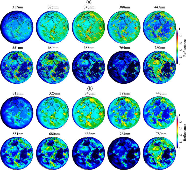
Figure 1. EPIC (a) observed and (b) synthetic reflectance images in 10 channels at 9:08 UTC, 2016 April 5.
Download figure:
Standard image High-resolution image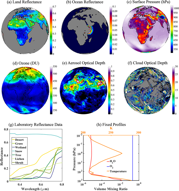
Figure 2. (a) Land reflectance map, calculated using the Ross–Thick–Li–Sparse model (Roujean et al. 1992). (b) Ocean reflectance map, calculated using the Cox–Munk model (Cox & Munk 1954). (c) Surface pressure map. (d) Column integrated ozone map. (e) Total aerosol optical depth map. (f) Total cloud optical depth. (g) Laboratory reflectance data for seven surface types. Snow (300 ∼ 340 nm) and wetland (300 ∼ 400 nm) reflectance are partly extrapolated in the UV channels, using the nearest available value. Wetland, shrub, snow, lichen, and grass data are taken from the USGS Spectral Library (Kokaly et al. 2017). Desert and tree data are from the RELAB spectral database (Pieters & Hiroi 2004). (h) Fixed vertical profiles used for water vapor, oxygen, and temperature. All maps are for the 551 nm channel and have the same viewing geometry of EPIC at 9:08 UTC, 2016 April 5.
Download figure:
Standard image High-resolution image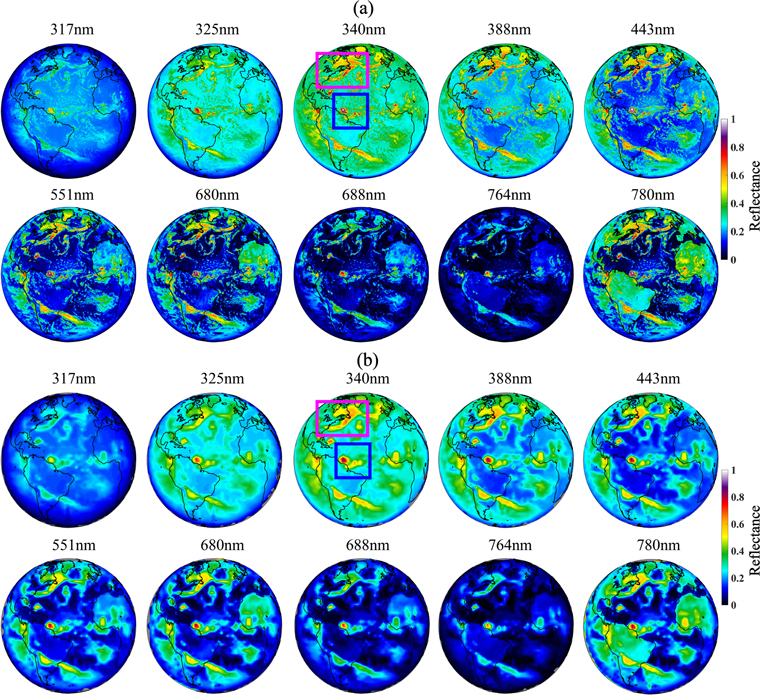
Figure 3. EPIC (a) observed and (b) synthetic reflectance images in 10 channels at 14:47 UTC, 2016 August 7. The purple and blue boxes indicate examples of midlatitude front and tropical deep convective cloud, respectively.
Download figure:
Standard image High-resolution imageTable 1. Surface Type Categorization
| Index | Surface Type | Index | Surface Type | ||
|---|---|---|---|---|---|
| Tree | 1 | Evergreen Needleleaf Forest | 12 | Cropland | |
| 2 | Evergreen Broadleaf Forest | 14 | Croplands Mosaics | ||
| 3 | Deciduous Needleleaf Forest | Wetland | 11 | Permanent Wetlands | |
| 4 | Deciduous Broadleaf Forest | Lichen | 18 | Tundra | |
| 5 | Mixed Forest | Desert | 13 | Urban and Built-up | |
| Shrub | 6 | Closed Shrublands | 16 | Bare Soil and Rocks | |
| 7 | Open Shrublands | Ocean | 17 | Water Bodies | |
| Grass | 8 | Woody Savannas | Snow/Ice | 15 | Snow and Ice (permanent) |
| 9 | Savannas | 19 | Snow (seasonal over land) | ||
| 10 | Grasslands | 20 | Ice (on water bodies) | ||
Note. The 19 land surface types in the DSCOVR composite data are regrouped into seven.
Download table as: ASCIITypeset image
The water surface reflectance in ESS is simulated by the Cox–Munk model (Cox & Munk 1954). It enables the calculation of liquid water specular reflectance given wind speed and water refractive index, and thus can reconstruct the sunglint feature (Figure 2(b)). The input wind speed data is also obtained from DSCOVR composite data (NASA/LARC/SD/ASDC 2017). Due to spatial degradation, coastal pixels are mixtures of both land and ocean surfaces. For these pixels, RT calculations are performed twice, once each for land and ocean surface. The radiance is calculated as a weighted average based on the area fractions of the original land and ocean pixels.
2.3. Atmospheric Properties
Both Rayleigh scattering and molecular absorption are included in ESS. Given the fact that EPIC bands are narrow, contributions from gaseous species other than O2, O3, and H2O are small; therefore, only these three gases are considered in the EPIC simulations (Table 2). For O2, and H2 O, gas absorption cross-sections are generated using the HITRAN 2008 database (Rothman et al. 2009), on top of which additional continuum absorption is also included using the MT_CKD model (Mlawer et al. 2012). The HITRAN-based cross-sections are calculated as Voigt line profiles using the pressures and temperatures of the respective atmospheric layers. For O3, cross-section tables based on the works of Daumont et al. (1992), Brion et al. (1993), Brion et al. (1998), and Malicet et al. (1995) are used. Moreover, H2O and temperature profiles are assumed to be spatially invariant due to their limited effect on the light curves (Figure 2(h)). Also, as O2 is well-mixed in the Earth's atmosphere, a uniform vertical distribution is employed over the entire Earth (Figure 2(h)). The representative profiles shown in Figure 2(h) are extracted over the land region (34°N) at noontime in the US from the National Center for Environmental Prediction–National Center for Atmospheric Research reanalysis data (Kalnay et al. 1996). The spatially and temporally varying surface pressure (Figure 2(c)) data are extracted from the Modern-Era Retrospective analysis for Research and Application, Version 2 (MERRA-2; Global Modeling & Assimilation Office 2015b). For each pixel, the a priori temperature and H2O profiles (Figure 2(h)) are interpolated to the MERRA-2 pressure levels in log-pressure space for the RT calculation. ESS also uses spatially and temporally varying three-dimensional O3 data, similarly extracted from MERRA-2 (Global Modeling & Assimilation Office 2015b; Figure 2(d)), which provides 3 hourly, instantaneous assimilations of ozone mixing ratio in 72 model layers. For the purpose of reasonably reducing computation and storage cost, we use data on days 5, 15, and 25 of each month in lieu of a fully varying data set.
Table 2. Gaseous Absorption
| Band Index | Band Center (nm) | O2 (CTM a ) | O2 | O3 | H2 O (CTM) | H2O |
|---|---|---|---|---|---|---|
| 1 | 317 | ✓ | ||||
| 2 | 325 | ✓ | ||||
| 3 | 340 | ✓ | ✓ | |||
| 4 | 388 | ✓ | ✓ | |||
| 5 | 443 | ✓ | ✓ | |||
| 6 | 551 | ✓ | ✓ | ✓ | × | |
| 7 | 680 | ✓ | ✓ | × | ||
| 8 | 688 | × | ✓ | ✓ | × | |
| 9 | 764 | ✓ | × | ✓ | × | |
| 10 | 780 | × | ✓ | ✓ | × | |
Notes. Cross marked area denotes the use of the HITRAN 2008 database, while right mark indicates that cross-section tables are used.
a CTM denotes continuum absorption.Download table as: ASCIITypeset image
The atmospheric aerosol data is also extracted from the MERRA-2 data set (Global Modeling & Assimilation Office 2015a), which provides mixing ratios in 72 model layers for five aerosol types: dust, sulfate, sea salt, black carbon, and organic carbon. The wavelength-dependent scattering and extinction coefficients and phase functions of these aerosol types are calculated using Mie scattering theory, except for dust where nonsphericity is taken into account (Meng et al. 2010). The aerosol optical properties are obtained using the same methodology as that used by Crisp et al. (2021). Figure 2(e) shows an example of the total aerosol optical depth distribution in the 551 nm channel. Similar to the procedure for O3, data on days 5, 15, and 25 of each month are used in the analysis.
Clouds constitute another important contribution to the UV-NIR Earth spectrum. We classify clouds as liquid and ice particles. For simplicity, only one type of cloud is assumed to exist at a single pixel and the vertical distribution is prescribed and fixed. Liquid cloud optical properties are computed using Mie theory, with parameters relevant to continental stratus clouds employed in the calculations (Hess et al. 1998). For ice clouds, a habit mixture of generalized cirrus is assumed (Baum et al. 2011). The cloud spatial distribution, optical depth, effective pressure, and effective radius (for ice clouds only) are obtained from EPIC composite data (NASA/LARC/SD/ASDC 2017). A sample total cloud optical depth distribution map is shown in Figure 2(f). Multiple RT computations are performed for degraded pixels with mixed cloud types at the degraded spatial resolution. For example, the simulated reflectance of a pixel covered with 50% liquid cloud, 20% ice cloud, and 30% clear sky is computed using a weighted average of three separate RT calculations.
3. Results
Figures 1(b) and (b) show examples of simulated Earth images in the 10 EPIC channels at two time points. ESS is able to reproduce all major characteristics in the observations. Generally, in the shortest wavelength channels, the strong Rayleigh scattering results in bright images. Due to the increasing ozone absorption from 340 to 317 nm, the brightest image is in the 340 nm channel (Figures 1 and 3). On the other hand, in the longer wavelength channels, surface information is more clearly seen except for the two oxygen absorption channels (688 and 764 nm). An enhancement of land reflectance is apparent, especially for vegetated pixels (Appendix A1) because of the red edge effect (Figures 1 and 3; 780 nm). Owing to the detailed description of land BRDF, the reflectance features of different land surface types are reflected in the simulations; for example, the increasing reflectance of desert pixels (Appendix A1) through the 551, 680, and 780 nm channels, in contrast with the abrupt increase of vegetation reflectance in the 780 nm channel. Moreover, the usage of MAIAC data (NASA/LARC/SD/ASDC 2018) guarantees a better representation of the backscattering peak viewed at EPIC geometry. The ocean glint feature can also be seen due to the inclusion of the Cox–Munk surface model (Figures 1(b) and 3(b)). The exact location and cloud characteristics are slightly different due to the usage of the DSCOVR composite data set (NASA/LARC/SD/ASDC 2017); the cloud data in the satellite composite data set is not at exactly the same time as the EPIC observations, but the general cloud patterns, such as tropical deep convective clouds (blue box in Figure 3) and midlatitude fronts (purple box in Figure 3) can still be captured at the degraded spatial resolution.
The differences between the ESS results and the observations suggest possible improvements. First, in the short wavelength channels, simulated reflectances for clear-sky pixels are lower than observed values. This is possibly a result of the simplified treatment of multiple scattering in the 2S-ESS model. Cloudy pixels generally appear to be brighter in the simulations, especially those with ice clouds. This could be a result of both simplified ice cloud models and degraded cloud properties due to the low spatial resolution used in the simulations. Also, snow- or ice-covered pixels are darker due to the Lambertian assumption. However, this has a small effect in the simulations due to the low spatial coverage (∼10%) and confinement to high latitudes, which have small weights in disk integration. Extreme viewing geometry can also cause problems at the edges of the disk.
A comparison of the time-averaged Earth spectrum between EPIC observations and simulations is shown in Figure 4. The same time points are used in both data sets to calculate the time-averaged reflectance. ESS reproduces the mean Earth spectrum with errors less than 7% (Table 3), and mostly within 5%, except for the two oxygen absorption channels (688 and 764 nm), where the simulations are brighter than the observations by as much as 19.53%. For bands 317–443 nm, ESS provides a slightly darker simulation, while for the other longer wavelength channels, the simulation tends to be brighter. The standard deviation in each channel is denoted in Figure 4 by the shaded area, and the percentage difference in reflectance between the two data sets is shown in Table 3. In general, the simulated data show a slightly larger temporal variation than the observations. A comparison between the simulated and observed light curves in the 10 channels is shown in Figure 5. Time-averaged values are extracted from both data sets in all channels. A general seasonal cycle with a larger reflectance during the southern hemisphere summer, which is related to a closer Sun–Earth distance and the Antarctic ice sheet, can be reproduced by the simulations in all the channels. In addition, a relatively smaller enhancement during the northern hemisphere summer can also be seen in the simulations, which can be related to larger land cover and larger cloud cover due to the South Asian monsoon, as presented in Jiang et al. (2018). A scatter plot of the data points in Figure 5 is shown in Figure 6. The simulations show a good fit with the observations, with slopes all close to unity. Slightly larger slopes can be seen in the two oxygen absorption channels (688 and 764 nm). Table 3 shows the root-mean-square errors (RMSE) of the light curves presented in Figures 5 and 6, which helps to measure the goodness of the simulated time-dependent variability in each channel. With RMSE all smaller than 1%, the simulations show a good temporal match with the observations.

Figure 4. Time-averaged Earth spectrum. The red and blue lines represent the observed and simulated results, respectively. The shaded area denotes the standard deviation in each channel.
Download figure:
Standard image High-resolution image
Figure 5. Time series of disk-integrated reflectance deviation from the time average. Red and blue lines denote observed and simulated results, respectively.
Download figure:
Standard image High-resolution image
Figure 6. Correlation between simulated and observed disk-integrated reflectance deviations. The x- and y-axis values correspond to the observations and simulations, respectively, which are also the red and blue lines in Figure 5, respectively. The gray line denotes a 1:1 correspondence.
Download figure:
Standard image High-resolution imageTable 3. Model Performance
| Band Center (nm) | Avg Diff (%) | Std a Diff (%) | RMSE b (%) | Band Center (nm) | Avg Diff (%) | Std Diff (%) | RMSE (%) |
|---|---|---|---|---|---|---|---|
| 317 | −3.83 | 5.07 | 0.25 | 551 | 2.07 | 9.20 | 0.60 |
| 325 | −0.06 | 12.56 | 0.38 | 680 | 6.90 | 2.00 | 0.74 |
| 340 | −2.16 | 12.03 | 0.44 | 688 | 14.20 | 27.15 | 0.65 |
| 388 | −0.30 | 12.56 | 0.44 | 764 | 19.55 | 36.82 | 0.54 |
| 443 | −0.84 | 11.17 | 0.49 | 780 | 6.50 | −7.97 | 0.82 |
Notes. Negative values indicate that the simulation has a smaller result than the observation.
a Std denotes standard deviation. b RMSE denotes root-mean-square errors. For residual light curves, it is calculated by comparing the simulation to the observation in each channel over the entire time period.Download table as: ASCIITypeset image
To evaluate the performance of ESS in terms of capturing the spectral and time-dependent characteristics of the Earth in its disk-integrated light curves, we use singular value decomposition (SVD) analysis, in line with previous efforts (Fan et al. 2019; Gu et al. 2021), and compare the principal components (PCs) between observation and simulation (Figure 7). The entire observation data set contains ∼5000 time points in the year 2016, while the subsampled data set contains ∼300 time points to match the simulation. First, the comparison of the singular value distributions of the full and subsampled observation data sets suggests that ∼300 time points are sufficient to recover the time variation characteristics of the light curves, although the singular values are smaller in amplitude due to fewer time points (Figure 7(a)). Second, for the same time points, the singular values of the simulated light curves are generally larger than those of the subsampled observations, corresponding to larger temporal variation in the simulated light curves (Table 3). For both data sets, the first two PCs (PC1 and PC2) contribute more than 95% of the total variance, while the last four PCs (PC7 to PC10) contribute less than 0.3%. Therefore, we ignore the latter in the PC spectra comparison (Figure 7(b)). The sequence of the observed PC spectra is adjusted for a clearer comparison of their characteristics; specifically, PC3 and PC4 are switched. The simulation successfully reconstructs PCs 1–5. In particular, for the first two PCs, the simulation has a near perfect match with the observation, indicating that ESS can recover the two most important signals, which have previously been reported as indicative of low clouds and surface distribution, respectively (Gu et al. 2021). The observed PC4 and PC3 also have good matches with the simulated PC3 and PC4. Since the observed PC4 mainly contains high cloud information (Gu et al. 2021) and ESS simulates the high (ice) clouds with a brighter reflectance, the eigenvalue of this signal increases along with increased variance contributed by high clouds.
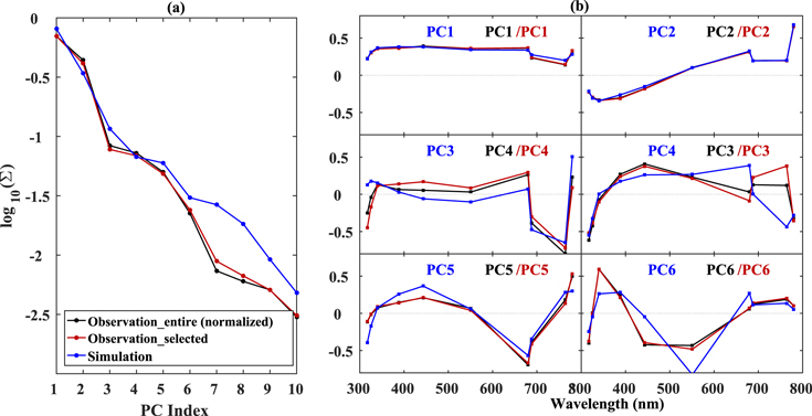
Figure 7. (a) Singular values for the full observation (black; ∼5000 time points; normalized by a factor of 0.26), subsampled observation (red; ∼300 time points, same as the number of simulation time points), and simulated (blue) light curves. (b) Eigenvectors (spectra) of the first six PCs of the full observation (black), subsampled observation (red), and simulated (blue) light curves. The text in each panel denotes the PC index for the three sets of data. PC3 and PC4 are switched between the simulations and observations for a clearer comparison.
Download figure:
Standard image High-resolution image4. Discussion
ESS is capable of reproducing EPIC observations in the 10 wavelength channels, in terms of both absolute brightness and temporal variation. It can also reconstruct the principal components, which represent the spectrophotometric variations of the Earth. This validation not only ensures the accuracy of ESS as a tool for producing EPIC-like data for further research related to EPIC observations, but also hints at the potential for extending it to other wavelengths. Furthermore, because of the detailed treatment of the directional reflection of the surface, it enables a new generation of more realistic phase-dependent light curves of the Earth, which will extend the usage of EPIC observations for exoplanet research. Moreover, in comparison with the simplified model presented in Gu et al. (2021), the inclusion of RT processes enables ESS to simulate light curves of Earth-like exoplanets with different configurations, such as surface distribution, cloud patterns, and atmospheric conditions, in combination with general circulation models (GCMs). The Earth simulations provide a starting point and benchmark for characterizing exoplanets, especially in terms of utilizing temporal variations. Furthermore, for future missions aiming at the detection of Earth-like exoplanets, more emphasis will be placed on wavelengths from the UV to the NIR due to low planetary temperatures, such as the 575, 660, 730, and 825 nm bandpasses for the coronagraph instrument onboard the Nancy Grace Roman Space Telescope (Groff et al. 2021), the coronagraph and starshade instrument covering 0.2–1.8 μm on HabEx (Gaudi et al. 2019), and the ECLIPS instrument covering 0.2–2.0 μm on LUVOIR (Fischer et al. 2019). Combined with instrument models, ESS will be a good testing ground, generating Earth-like exoplanet light curves for detectability research.
Although our simulations provide good agreement with the observations, there are two possible improvements that can be implemented in future work:
(1) The simplified cloud settings account for a large part of the biases in the simulations. First, clouds (especially ice clouds) generally appear brighter in our simulations. Figures 8 and 9 show the probability distributions of the pixel reflectance for liquid and ice clouds, respectively. Both simulation and observation results are shown in all 10 channels for comparison. We select the liquid/ice cloud pixels based on the DSCOVR composite data, using a threshold of 80% in cloud fraction. The observations are all first degraded to the same spatial resolution as the simulations before selecting the pixels. For liquid clouds, a slightly longer tail of bright reflectance is noticeable in most of the channels; this is especially true in the longest four wavelength channels, where there is a clear shift of the distribution peak toward larger values (Figure 8). On the contrary, although there is no large shift of the peak in the ice cloud reflectance distribution, a fatter tail of high-reflectance values is evident in all channels, demonstrating a biased representation of ice cloud properties. Our knowledge of ice clouds is limited due to large uncertainties in ice crystal microphysical and optical properties. At the same time, sophisticated ice cloud models are being developed for various applications. A more meticulous classification and application of ice cloud models may help improve the current model. Second, the largest difference exists in the two oxygen absorption channels (688 and 764 nm) in both disk-integrated (Figures 4 and 6) and pixel (Figures 8 and 9) reflectance comparisons. Given the large sensitivity of these two channels to cloud height (Richardson et al. 2017; Zeng et al. 2020), we perform a sensitivity test by placing the clouds at 10% higher effective pressure. About 30 time points are tested, with both disk-integrated and pixel reflectance results shown in Figure 10. For a clearer comparison, results for the same time points in the original simulation are also shown. The average simulation difference drops by 4.62% and 7.86% in the 688 nm and 764 nm channels, respectively (Figure 10(a)), with no significant changes identified in the slopes. Since ice cloud effective pressure is generally smaller, a 10% increase would result in a smaller absolute change than that for liquid clouds. As a result, a relatively smaller shift to lower values can be found in the ice cloud pixel reflectance histograms (Figure 10(b)). Meanwhile, for liquid clouds, the peaks shift to smaller values with 9.86% and 14.27% decreases in average reflectance for 688 nm and 764 nm, respectively (Figure 10(c)). This demonstrates the importance of accurate cloud vertical distribution information.

Figure 8. Histograms of liquid cloud-covered pixel reflectance for observation (red) and simulation (blue) for the 10 EPIC channels.
Download figure:
Standard image High-resolution image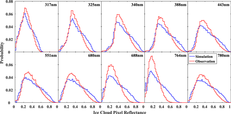
Figure 9. Same as Figure 8, but for ice cloud-covered pixels.
Download figure:
Standard image High-resolution image
Figure 10. (a) Scatter plots of simulated disk-integrated reflectance against observations for the original simulation (blue dots) and the "10% higher cloud effective pressure" experiment (red dots) in the two oxygen absorption channels. Linear regression results for the original simulation (blue line) and the experiment (red line) are also given. (b) Histograms of ice cloud-covered pixel reflectance for the original simulation (blue) and the experiment (red). (c) Same as (b), but for liquid cloud-covered pixels.
Download figure:
Standard image High-resolution image(2) Though the model gives good fits for the time-averaged reflectance in the short wavelength channels, the clear sky pixels are generally darker, compensating for the brighter clouds. As shown in Figure 11, a shift of the peak to smaller values becomes more significant in the shorter wavelength channels (pixels with a total cloud fraction less than 20% are selected). Given the strong Rayleigh scattering effect in these bands, the simplified multiple scattering approximation in the 2S-ESS RT model is likely the major cause of the relatively dark simulations. To demonstrate this effect, we compare results using the numerically more exact VLIDORT RT model (16 streams; Spurr 2006) with those from the 2S-ESS model, with gas absorption neglected. Comparisons for the 317 nm and 443 nm channels are shown in Figure 12. Despite the relatively small changes in cloud reflectance, the clear sky pixel reflectances in these two channels using VLIDORT are 22.32% and 59.34% larger on average than those using 2S-ESS, indicating the necessity for better representation of multiple scattering when simulating UV channels. Besides Rayleigh scattering, other factors such as ocean volume scattering and ocean color change due to chlorophyll may also contribute to the differences.

Figure 11. Same as Figure 8, but for clear-sky pixels.
Download figure:
Standard image High-resolution image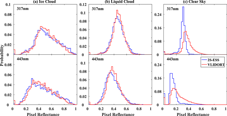
Figure 12. Histograms of (a) ice cloud-covered, (b) liquid cloud-covered, and (c) clear sky pixel reflectance for simulations using approximate (2S-ESS; blue) and numerically exact (VLIDORT; red) RT models.
Download figure:
Standard image High-resolution imageFurthermore, there are two more aspects that should be noted when using ESS for exoplanet characterization, especially when the focus is on atmospheric effects on light curves:
(1) Although the HITRAN 2008 database is used in the current version of ESS, inclusion of the latest HITRAN 2020 database, which contains more absorption lines for H2O and O2, introduces small differences in the absolute value of the simulated EPIC channel reflectance. A comparison of the transmissivity of H2O and O2 using the two databases in the five longest wavelength channels (the HITRAN database is only used for optical depth computations in these channels) is shown in Appendix A2. The profiles in Figure 2(h) are used to calculate the column integrated optical depth (OD), and the wavelength-dependent transmissivity is then calculated as exp(–OD). After convolution with filter functions, we can obtain the band-averaged transmissivities (Appendix A2). Compared to HITRAN 2008, HITRAN 2020 introduces small changes in the O2 transmissivity: there is a high bias of ∼ 0.23% in the 688 nm channel, and a low bias of ∼ 0.5% in the 764 nm channel. The greater number of H2O lines included in HITRAN 2020 results in smaller transmissivity in all five channels. However, as the H2O ODs are small, the updated HITRAN version has a negligible effect on the transmissivity, with changes ~ 0.01%. Table 4 provides a summary of the average reflectance difference between the HITRAN versions. We select eleven different sets of profiles (Figure A2; no aerosols or clouds), and calculate the one-dimensional reflectance over three different underlying surface types (forest, desert, and ocean) for multiple viewing geometries. The differences for the various scenarios in the 551 nm channel are also shown in Figure A3. The average difference for the 551 nm channel, shown in Table 4, is calculated by averaging all the data points (11 profiles, three surface types, and eight geometries) in Figure A3. The largest difference, caused by the O2 OD increase, is in the 764 nm channel, with ∼ 1.2% decrease in reflectance. For the other channels, the differences are within 0.5%, which demonstrates that usage of HITRAN 2020 would likely only result in small changes in the EPIC reflectance images.
Table 4. Average Reflectance Difference Between HITRAN 2020 and HITRAN 2008
| Band Center (nm) | Average Difference (%) a | Band Center (nm) | Average Difference (%) |
|---|---|---|---|
| 551 | −0.02 | 764 | −1.2 |
| 680 | −0.02 | 780 | −0.02 |
| 688 | 0.43 |
Notes. Negative values indicate that HITRAN2020 has a low bias in reflectance compared to HITRAN2008.
a Average difference is calculated by averaging the differences over all tested data points (11 profiles, three surface types, and eight solar zenith angles); an example for the 551 nm band is shown in Figure A3.Download table as: ASCIITypeset image
(2) In our current version of ESS, single representative temperature and H2O profiles are used for the entire Earth. Spatially and temporally varying profiles would likely cause changes in the disk-integrated reflectance. About thirty time points are tested with profile data from MERRA-2 (Global Modeling & Assimilation Office 2015c); the differences are shown in Table 5. The average differences in all channels are within 0.7%, which demonstrates a negligible influence of the variability in the profiles on the absolute disk-integrated reflectance. Moreover, the range of the differences, represented by the minimum and maximum values in Table 5, are all within 2%, which indicates small changes due to the temporal variation as well. It seems that integrating over the entire disk makes the spatiotemporal variation of temperature and H2O profiles a second or higher order effect on the light curves.
Table 5. Disk-integrated Reflectance Difference Caused by Spatially and Temporally Varying Temperature and H2O Profiles
| Band Center (nm) | Difference (%) Avg (Min, Max) a | Band Center (nm) | Difference (%) Avg (Min, Max) |
|---|---|---|---|
| 317 | −0.60 [−0.82, −0.37] | 551 | −0.21 [−0.32, −0.08] |
| 325 | −0.70 [−0.85, −0.55] | 680 | −0.11 [−0.32, 0.26] |
| 340 | −0.66 [−0.79, −0.54] | 688 | 0.15 [−0.11, 0.55] |
| 388 | −0.55 [−0.68, −0.44] | 764 | 0.68 [−0.07, 1.83] |
| 443 | −0.44 [−0.56, −0.36] | 780 | −0.08 [−0.11, −0.00] |
Notes. Negative values indicate that the varying profiles cause a decrease in reflectance.
a Average [Minimum, Maximum].Download table as: ASCIITypeset image
However, for future exoplanet characterization extending to other wavelength channels, the above effects may need to be considered.
5. Conclusions
We have developed a whole-disk spectral model, called ESS, to simulate light curves of the Earth and validated it using EPIC observations covering the spectral region from the UV to the NIR. The simulator utilizes the 2S-ESS line-by-line RT model and accounts for atmospheric effects, including clouds, aerosols, and gas absorption. Realistic surface contributions are also included by using appropriate BRDF data. We simulate ∼300 full-phase images in each channel for the year 2016 with a spatial resolution of ∼2000 pixels over the sunlit disk. The time-averaged spectrum, as well as the light curves, can be reproduced with high fidelity by ESS. The principal components can also be simulated, indicating the good performance of our model in reconstructing the temporal variation of the light curves. The largest discrepancies are in the two oxygen absorption channels (688 and 764 nm) for both the time-averaged reflectance and its temporal variation. These differences result from simplified cloud settings, especially for ice clouds, demonstrating the important role of clouds in determining the nature of disk-integrated light curves in gas absorption channels. In spite of these discrepancies, high cloud information can still be disentangled through SVD analysis, indicating the robustness of this signal. The simplified treatment of multiple scattering in the 2S-ESS RT model counteracts biases in cloud simulation in the UV channels. We envisage future improvements to better represent the multiple scattering contributions. The reproduction of Earth's characteristics (spectral and temporal) with high fidelity indicates that ESS can not only be used to generate Exo-Earth light curves but also be a testing ground for Earth-like exoplanet light curves in combination with GCMs. Moreover, combined with direct imaging instrument models, ESS can serve as a robust, reliable, and efficient forward model for future exoplanet characterizations.
This work was supported by the National Natural Science Foundation of China under grant 41888101. All computations were done at the High-performance Computing Platform of Peking University. A portion of this research was carried out at the Jet Propulsion Laboratory, California Institute of Technology, under a contract with the National Aeronautics and Space Administration (80NM0018D0004). Y.L.Y. was supported in part by a Virtual Planetary Laboratory grant from the University of Washington. S.F. acknowledges funding support from CNES. We acknowledge funding support from the NASA Exoplanet Research Program NNH18ZDA001N.
Appendix:
A1.
Eight surface types are included in our surface reflectance calculation (Figure A1).

Figure A1. Distribution of the eight surface types at (a) 9:08 UTC, 2016 April 5, and (b) 14:47 UTC, 2016 August 7.
Download figure:
Standard image High-resolution imageA2.
In order to illustrate the differences between HITRAN 2008 and HITRAN 2020, we provide the transmissivity of H2O and O2, calculated using the two databases in the five longest wavelength channels, in Table A1. Further, eleven different sets of profiles (Figure A2; no aerosols or clouds) are used to calculate the one-dimensional reflectance over three different underlying surface types (forest, desert, and ocean) for multiple viewing geometries. An example of the reflectance difference is shown for the 551 nm channel in Figure A3.
Table A1. Sample Transmissivities for H2O and O2 Calculated using HITRAN 2008 and HITRAN 2020
| Band Center (nm) | H Transmissivity a (%) | O2 Transmissivity (%) | ||
|---|---|---|---|---|
| HITRAN 2008 | HITRAN 2020 | HITRAN 2008 | HITRAN 2020 | |
| 551 | 99.9557 | 99.9433 | 100.00 | 100.00 |
| 680 | 99.9664 | 99.9622 | 99.8404 | 99.8420 |
| 688 | 99.8210 | 99.8159 | 71.2951 | 71.5293 |
| 764 | 100.00 | 99.9959 | 49.2614 | 48.7703 |
| 780 | 99.9733 | 99.9659 | 99.9998 | 99.9998 |
Note.
a The Transmissivity is calculated as exp(–OD), where the OD denotes the column integrated optical depth. The profiles used in the OD calculations are shown in Figure 2(h). The values of band-averaged transmissivity, shown in the table, are after convolution with the filter function for each band.Download table as: ASCIITypeset image
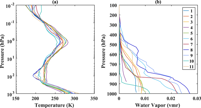
Figure A2. Profiles of (a) temperature and (b) H2O used for the reflectance comparison between HITRAN 2008 and HITRAN 2020.
Download figure:
Standard image High-resolution image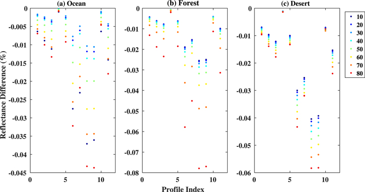
Figure A3. Reflectance difference between HITRAN 2020 and HITRAN 2008 in the 551 nm channel. Tests are done for the eleven different sets of profiles shown in Figure A2, over three different underlying surface types: (a) ocean, (b) forest, and (c) desert. For each set of profiles over each underlying surface type, eight different viewing geometries are tested (colored dots): solar zenith angle (equal to viewing zenith angle) varies from 10°to 80°. The relative azimuth angle is assumed to be 170°.
Download figure:
Standard image High-resolution image