


Abstract
I assemble 4684 star-forming early-type galaxies (ETGs) and 2011 composite ETGs (located in the composite region on the BPT diagram) from the catalog of the Sloan Digital Sky Survey Data Release 7 MPA-JHU emission-line measurements. I compare the properties of both ETG samples and investigate their compositions, stellar masses, specific star formation rates (sSFRs), and excitation mechanisms. Compared with star-forming ETGs, composite ETGs have higher stellar mass and lower sSFR. In the stellar mass and u − r color diagram, more than 60% of star-forming ETGs and composite ETGs are located in the green valley, showing that the two ETG samples may have experienced star formation and that ∼17% of star-forming ETGs lie in the blue cloud, while ∼30% of composite ETGs lie in the red sequence. In the [N II]/Hα versus EWHα (the Hα equivalent width) diagram, all star-forming ETGs and most of the composite ETGs are located in the star-forming galaxy region, and composite ETGs have lower EWHα than their counterparts. We show the relations between 12+log(O/H) and log(N/O) for both ETG samples, and suggest that nitrogen production of some star-forming ETGs can be explained by the evolution scheme of Coziol et al., while the prodution of composite ETGs may be a consequence of the inflowing of metal-poor gas and these more evolved massive galaxies.
Export citation and abstract BibTeX RIS

Original content from this work may be used under the terms of the Creative Commons Attribution 4.0 licence. Any further distribution of this work must maintain attribution to the author(s) and the title of the work, journal citation and DOI.
1. Introduction
Lenticular and elliptical galaxies constitute early-type galaxies (ETGs), and the traditional picture of ETGs is "red and dead" without any star formation (SF). Using the galaxy optical colors of the Sloan Digital Sky Survey (SDSS) data, Strateva et al. (2001) described that the distribution of galaxies in the color–color diagram is bimodal. Analyzing the bivariate distribution from the SDSS data in the color–magnitude diagram, it was established that red optical colors and blue colors are located in a tight red and blue sequence (Baldry et al. 2004).
The color of galaxies is correlated with galaxy morphology. In the local universe, the color divides galaxies into two different types of groups superposed in the color–magnitude diagram: blue cloud galaxies are less massive and are actively star-forming, while red sequence galaxies tend to be massive and be dominated by old stars (Brinchmann et al. 2004; Wyder et al. 2007; Taylor et al. 2009). ETGs have long been regarded as the endpoint of galaxy evolution. Galaxy evolution, from the blue cloud location of star-forming galaxies (SFGs) to the red sequence, happens through the green valley (GV) transition in the color–magnitude diagram (Martin et al. 2007).
Many studies find recent or ongoing SF in some ETGs, and focus on explaining the SF. The fuel for the SF may be provided via minor/major mergers (Naab et al. 2009; Kaviraj et al. 2013) and/or low-metallicity gas accretion (lucero & Young 2007; Serra et al. 2012). Minor mergers tend to be frequent at low redshift, while major mergers are more usual at high redshift (George 2017).
The mergers and inflowing of metal-poor gas can bring gas and trigger SF. In cosmological models, the merging process is a natural phenomenon, plays an important role for the assembly of massive galaxies (e.g., Kauffmann 1996), and shows that elliptical galaxies are the most massive objects. Utilizing near-ultraviolet (NUV)/optical data of NGC 4150 from the Wide-Field Camera 3 on the Hubble Space Telescope, Crockett et al. (2011) demonstrated that recent SF is fueled by a large reservoir of molecular gas, which originated mainly from the infalling companion of a minor merger and they suggested that the SF contributes ∼2%–3% of the galaxy stellar mass. Similarly, Kaviraj (2014) used ∼6500 galaxies to estimate a fraction of cosmic SF triggered by minor mergers and found that ETGs contribute at least ∼14% of the cosmic SF budget. Employing numerical simulations to analyze the relation between SF enhancement and galaxy interaction, Di Matteo et al. (2008) suggested that some major mergers can result in a strong starburst. With regard to major-merger-driven SF, major mergers can provide about 27% of the SF budget in 80 massive galaxies at z ∼ 2 (Kaviraj et al. 2013). Based on photometric and spectroscopic observations of the Hoag's object, Finkelman et al. (2011) showed the object formation does not attribute to merger events, and suggested that a "cold" accretion of the pristine material comes from the intergalactic medium (IGM).
In this study, I explore the properties of star-forming ETGs and composite ETGs, which lie in the H ii region of the [S II]/Hα versus [O III]/Hβ ([S II] Baldwin–Philips–Terevich (BPT) diagram, Baldwin et al. 1981) and the composite region of the [N II]/Hα versus [O III]/Hβ ([N II] BPT) diagram, respectively. The two types of ETGs are selected with the same judgment standard of ETGs, but they are located at different regions of the BPT diagram. Since they may possess different ionization mechanisms, we need to study various properties of the two types of ETGs and to compare differences between their various properties. I collected samples of star-forming ETGs and composite ETGs by utilizing the SDSS 7th Data Release (DR7) Max Planck Institute for Astrophysics—John Hopkins University (MPA-JHU) emission-line measurements and Galaxy Zoo 1 data in Section 2. In Section 3, the distributions of stellar mass and specific star formation rate (sSFR) for the two types of ETGs are displayed. I also compare the distributions of the two types of ETGs on the stellar mass and u − r color diagram, [N II]/Hα versus EWHα (the Hα equivalent width, WHAN) diagram, and stellar mass and SFR diagram. In addition, I present the mass–metallicity (MZ) relation, sSFR versus 12+log(O/H), and 12+log(O/H) versus log(N/O). In Section 4, I discuss the results, possible interpretations, and implications. In Section 5, I summarize the results.
2. The Data
In this paper, I compare various properties between composite ETGs and star-forming ETGs by utilizing the DR7 (Abazajian et al. 2009) of the SDSS. The SDSS data can supply a total of more than 900,000 galaxy spectra. The catalog of the MPA-JHU for the SDSS DR7 supplies the stellar mass (Kauffmann et al. 2003b), SFR (Brinchmann et al. 2004), emission-line fluxes, and EWHα , which are publicly available. 1
For the composite ETG sample, I employ the selection method of Wu (2020) and the color divisor of W2 − W3 = 2.0 between ETGs with and without SF (Wu 2021). For the star-forming ETG sample, I use the method of Vincenzo et al. (2016) to avoid a bias by using nitrogen-enriched H ii regions to select these ETGs. Next, I will introduce the method for selecting both ETG samples. To avoid the aperture bias of MZ relations (Kewley et al. 2005), I select these galaxies with 0.04 < z < 0.12. The aperture covering fraction is calculated from the Petrosian and fiber magnitudes in the r band and the parameter is required to have more than 20% for all galaxies. For all galaxies, I choose those with signal-to-noise ratio (S/N) > 2 for [O II]λ λ3227, 3229, and [N II] λ6584, and S/N > 3 for Hα and Hβ as our galaxies. An SFR FLAG keyword, showing the measurement status of SFRs, is required to be zero in the catalog. The initial sample comprises 140,589 galaxies.
For an ETG sample, I employ the two judgment standards to select ETGs (Wu 2020). The first criterion is that these galaxies should be nSersic > 2.5 and the second one is the elliptical probability (p, the debiasing procedure has been applied for all the probabilities in this work) of more than 0.5 (Herpich et al. 2018). The first parameter is the Sérsic index, which comes from the New York University Value-Added Galaxy Catalog 2 (NYU-VAGC; Blanton et al. 2005). The second parameter is a fraction of votes for each galaxy morphology, classified by citizen scientists in the DR1 of the Galaxy Zoo project (Lintott et al. 2008, 2011). I first use the initial sample to cross match the NYU-VAGC within 2'', and have the demand of nSersic > 2.5 for these galaxies. Then I require these galaxies to satisfy p > 0.5 (Herpich et al. 2018) and utilize Table 2 of Lintott et al. (2011) to match my galaxies within 2''. As a result, I obtain a sample of 16,623 ETGs.
I have two conditions for selecting star-forming ETGs: (1) the Kewley et al. (2001) demarcation lines in the [S II] BPT diagram (Belfiore et al. 2015; Sánchez et al. 2015; Vincenzo et al. 2016), and (2) the Hα equivalent width (EWHα ) of > 6 Å (Cid Fernandes et al. 2010). Here, I obtain 4684 star-forming ETGs. When p > 0.8, a sample of 1760 star-forming ETGs is acquired. For composite ETGs, I use the Kauffmann et al. (2003a) and Kewley et al. (2001) curves to select them on the [N II] BPT diagram and acquire 6048 composite ETGs. In addition, I get 2291 composite ETGs when p > 0.8. In Figure 1, we show our samples of 4684 star-forming ETGs and 6048 composite ETGs, which are represented by the blue and red dots, respectively. All star-forming ETGs lie in the H ii region of the [S II] BPT (see Figure 1(a)), while all composite ETGs are located only the composite region of the [N II] BPT (see Figure 1(b)). From Figures 1(a) and (c), we can see that most of the composite ETGs are located in the LINER region of the [S II] BPT and [O I] BPT diagrams and that a minority of them lie on the H ii region of the two BPT diagrams.
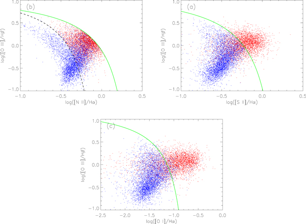
Figure 1. BPT diagnostic diagram. The black dashed curve shows the semi-empirical lower boundary for SFGs from Kauffmann et al. (2003a); the green solid curves represent the Kewley et al. (2001) theoretical upper limit for SFGs. The blue and red dots display star-forming ETGs and composite ETGs, respectively.
Download figure:
Standard image High-resolution imageBecause composite ETGs may have various ionization sources such as active galactic nuclei (AGNs), cosmic rays, and shocks, if we measure and study the metallicity of composite ETGs, we must select those ETGs with the dominant mechanism of SF. Because Kewley et al. (2001) established an extreme starburst line, which is the upper limit for SFGs on the [N II]/Hα versus [O III]/Hβ diagram and Griffith et al. (2019) suggested that these galaxies located below the curve were dominated by SF, I did not consider the contribution of AGNs on the ionization mechanisms of these galaxies for my analyses.
To explore further ionization sources of composite ETGs, I used the Wide-field Infrared Survey Explorer (WISE; Wright et al. 2010) catalog to research their possible photoionization. The survey covers the whole sky in four bands: W1, W2, W3, and W4, and their central wavelengths are 3.4, 4.6, 12, and 22 μm, respectively. The survey supplies four-band instrumental profile-fit photometry S/Ns, four-band instrumental profile-fit photometry magnitudes, the accurate position, and four-band fluxes, and these parameters are publicly available. 3 I select composite ETGs by cross matching the catalog of the ALLWISE sources within 2'' and by requiring S/N > 3 for W2 and W3.
Herpich et al. (2016) showed a finding that these galaxies with mid-IR color W2 − W3 > 2.5 present the presence of SF. From Figure 3 of Wu (2020), we can see that the diagnostic tool of W2 − W3 > 2.5 is used to select composite ETGs with SF. They suggested that the dominant excitation source is SF in these ETGs. In Wu (2021), 77,476 ETGs are used to explore the separator between ETGs with and without SF and they find that W2 − W3 = 2.0 is the best divisor for various ETGs. Therefore, here we employ the separator of W2 − W3 > 2.0 color to study our composite ETGs. In Figure 2, we show the W2 − W3 color histogram for the two types of ETGs. The blue dotted and red dashed lines represent the distributions of W2 − W3 of 4684 star-forming and 3259 composite ETGs, respectively. For star-forming ETGs, 4582 ETGs have W2 − W3 > 2.0, accounting for nearly 98% of 4684 ETGs. For composite ETGs, all ETGs have W2 − W3 > 2.0.
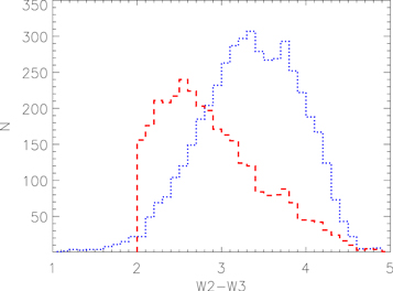
Figure 2. The distributions of W2 − W3 for star-forming ETGs and composite ETGs. The blue dotted and red dashed lines show their distributions for the two types of ETGs.
Download figure:
Standard image High-resolution imageIn addition, the issue of the ionized gas of various galaxies has been discussed in many recent papers, in particular, in the two recent reviews on the topic by Sánchez (2020) and Sánchez et al. (2021). Regarding the difficulty of identifying the ionized gas of ETGs, I use EWHα > 6 Å (Cid Fernandes et al. 2010) to obtain the two reliable ETG samples. In this work, I employ the method of Wu (2020) to exclude the following excitation mechanisms: shocks, PAGB stars, cosmic rays or extra heat (Belfiore et al. 2016; Griffith et al. 2019), [Ne iii]λ3869 photoionization transition (Athey & Bregman 2009), and single-degenerate SNe Ia progenitors (Woods & Gilfanov 2014; Griffith et al. 2019). Finally, I derive a sample of 2011 composite ETGs dominated by SF. Because these composite ETGs have an ionization mechanism dominated by SF activity, we may not assess the influence of other excitation sources on the ionization mechanism of these galaxies. Figure 3 shows the distributions of [N II]/Hα and EWHα from the WHAN diagram. The blue dotted and red dashed lines show their distributions of 4684 star-forming and 2011 composite ETGs with EWHα > 6 Å, respectively. Because these star-forming ETGs are derived using the [S II] BPT diagram including star-forming ETGs, some composite ETGs, and some ETGs located in the AGN region of the [N II] BPT diagram (see Figure 1(b); the percentages are about 56%, 41%, and 3%, respectively), there are are 1841 ETGs sources common to both the star-forming and composite ETG samples. In Figure 3(a), star-forming and composite ETGs have median values of [N II]/Hα ∼ − 0.35 and ∼−0.26, respectively. In Figure 3(b), the two types of ETGs present median values of EWHα ∼18.2 Å and ∼13.4 Å, respectively.

Figure 3. The distributions of [N II]/Hα and EWHα for star-forming and composite ETGs. The blue dotted and red dashed lines are the same as in Figure 2.
Download figure:
Standard image High-resolution imageThe measurements of M* (Kauffmann et al. 2003b) and SFRs (Brinchmann et al. 2004) are provided by the MPA-JHU catalog and these measurements are corrected by a Chabrier (2003) initial mass function (IMF) assuming a Kroupa (2001) IMF. In the samples of star-forming ETGs and composite ETGs, the two types of ETGs have the same photoionization source as SFGs, and we can use the abundance measurements of the extragalactic H ii region to calibrate their metallicities. In this paper, I estimate oxygen abundances of both ETG samples by using the R23 method (Pilyugin et al. 2006, 2010; Wu & Zhang 2013) and adopt the calibration of Tremonti et al. (2004; T04). In addition, I use a convenient formula of a five-level atom calculation of Pagel et al. (1992) to compute the N/O ratios for our ETGs (Wu & Zhang 2013)

where N2 = 1.33 [N II]λ6584, R2 = I[O II]λ3727+λ3729/IHβ
, and tII = 6065 + 1600x + 1878x3 + 2803x3 (x = log R23 = ![$\mathrm{log}({I}_{[{\rm{O}}\,{\rm\small{II}}]\lambda 3727+\lambda 3729+[{\rm{O}}\,{\rm\small{III}}]\lambda 4959+\lambda 5007}/{I}_{{\rm{H}}\beta })$](https://content.cld.iop.org/journals/1538-3881/163/1/28/revision3/ajac3484ieqn1.gif) ; Thurston et al. 1996).
; Thurston et al. 1996).
In addition, we estimate the dust-extinction-corrected u − r colors to investigate the positions of the two types of ETGs in the color-stellar-mass diagram. I execute k corrections to u- and r-band Petrosian magnitudes, subsequently performing Galactic extinction and internal corrections. First, the k corrections for the Petrosian magnitudes are based on the NYU-VAGC (Blanton & Roweis 2007). Then, I utilize the dust maps from Schlegel et al. (1998) to correct the foreground Galactic extinction. Finally, I correct the internal dust extinction by using the EBV_STAR values from the OSSY catalog (Oh et al. 2011) and the Calzetti et al. (2000) extinction law. I derive the Petrosian magnitudes of u and r bands for 4654 star-forming ETGs and 1993 composite ETGs.
3. Results
3.1. Sample Properties in the Two Types of Early-type Galaxies
For the two types of ETGs, I show their distributions of stellar mass and sSFR in Figure 4. The distributions of stellar mass for star-forming ETGs and composite ETGs are described, respectively, with blue dotted lines and red dashed lines. Compared to the stellar mass distribution of composite ETGs, the distribution of star-forming ETGs have a broader range. Composite ETGs have almost the same maximum of stellar mass as star-forming ETGs, while the minimum of stellar mass of the former ones is significantly higher than that of the latter ones. Star-forming ETGs have a median value of log (M*/M⊙) = 10.46, while the composite ETG sample has a median value of log (M*/M⊙) = 10.56, and the median value of the former is about 0.1 dex lower than that of the latter. We use the green solid and magenta dotted–dashed lines to show the distributions of their stellar masses for star-forming and composite ETGs with p > 0.8, respectively, and their median values are log (M*/M⊙) = 10.47 and log (M*/M⊙) = 10.55, respectively. From the comparison of the two median values of stellar masses of star-forming/composite ETGs with p > 0.5 and p > 0.8, we can see that star-forming or composite ETGs with p > 0.8 could not change our results when their stellar masses are compared. In addition, we find that the two samples of star-forming/composite ETGs with p > 0.5 and p > 0.8 have similar distributions. From comparisons of the median values of their stellar masses, we can see that composite ETGs have higher stellar masses than star-forming ETGs.

Figure 4. Comparison of stellar-mass (left-hand panel) and sSFR (right-band panel) distributions for star-forming ETGs and composite ETGs. The blue dotted and red dashed lines show the distributions of star-forming and composite ETGS, respectively. The green solid and magenta dotted–dashed lines present the distributions of star-forming and composite ETGs with p > 0.8, respectively.
Download figure:
Standard image High-resolution imageMoreover, Figure 4(b) displays the distributions of sSFR for the two types of ETGs. In this figure, the blue dotted lines and red dashed lines describe the distributions of sSFR for star-forming ETGs and composite ETGs, respectively. The median value of log(sSFR) for star-forming ETGs is − 10.09 yr−1, while − 10.30 yr−1 is the median value of the log(sSFR) of composite ETGs. From the maximum of their sSFR distributions, we can see that star-forming ETGs present clearly higher sSFR values. Compared to star-forming ETGs, composite ETGs have weaker SF activity. Compared with composite ETGs, star-forming ETGs have lower stellar mass and higher sSFR and star-forming and composite ETGs have different distributions of SFRs with median values of 0.32 M⊙ yr−1 and 0.26 M⊙ yr−1, respectively. The green solid and magenta dotted–dashed lines represent the distributions of sSFRs for star-forming and composite ETGs with p > 0.8, and the median values of their sSFRs are − 10.10 yr−1 and − 10.27 yr−1, respectively. From the comparison of the two median values of sSFRs for star-forming or composite ETGs with p > 0.5 and p > 0.8, we can see that ETGs with p > 0.5 do not influence our statistical results compared to ETGs with p > 0.8.
In Figure 5, we show the diagram of stellar mass and dust-corrected u − r color (from Petrosian magnitudes). The two green lines are Equations (1) and (2) of Schawinski et al. (2014), defining the green valley (GV) galaxies. The two green lines divide these ETGs into three parts (from bottom to top): a blue cloud, a GV, and a red sequence. The blue and red contours are the distributions of star-forming ETGs and composite ETGs, respectively. We can see that star-forming ETGs take up the entire u − r color range, while composite ETGs occupy mainly the GV and red sequence. Compared with star-forming ETGs, composite ETGs have redder color.
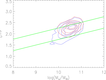
Figure 5. The diagram of stellar mass and corrected u − r color. The two green lines represent the position of the green valley, defined as the region between the blue cloud and the red sequence. The blue and red contours show the distributions of star-forming and composite ETGs, respectively.
Download figure:
Standard image High-resolution imageIn Table 1, I list the fraction of star-forming and composite ETGs that lie in the different regions of the stellar-mass–color diagram. From Table 1, we can see that more than 60% of star-forming and composite ETGs lie in the GV region in the stellar mass and u − r diagram. Star-forming ETGs do not completely enter into the GV zone, and the remaining ETGs are divided into a red sequence and a blue cloud with about a one-to-one ratio. These results show that star-forming ETG samples mainly lie in a transition state and have experienced higher SF activity in the past. Compared with star-forming ETGs, only 8% of composite ETGs are located in the blue cloud in Figure 5. Regarding a tail of ∼8% of the group reaching the blue sequence, this is very similar to the result (a few ETGs touching the blue cloud) of Schawinski et al. (2014), but their ETG population has a lower GV percentage than my composite or star-forming ETGs. I also show the distribution of star-forming/composite ETGs with p > 0.8 in the stellar mass and u − r color diagram and find that the two samples of star-forming/composite ETGs with p > 0.5 and p > 0.8 have the similar percentages in a blue cloud, a GV, or a red sequence (see Table 1). These results indicate that star-forming/composite ETGs with p > 0.5 do not change the statistical percentage for their compositions in the stellar mass and u − r color.
Table 1. Summary of Star-forming and Composite ETGs
| Galaxy | N | Percent |
|---|---|---|
| Sample | Population | |
| S-ETGs, all(p a > 0.5) | 4654 | 100% |
| S-ETGs, blue cloud | 781 | 17% |
| S-ETGs, green valley | 2950 | 63% |
| S-ETGs, red sequence | 923 | 20% |
| S-ETGs, all(p > 0.8) | 1750 | 100% |
| S-ETGs, blue cloud | 285 | 16% |
| S-ETGs, green valley | 1119 | 64% |
| S-ETGs, red sequence | 346 | 20% |
| C-ETGs, all(p > 0.5) | 1993 | 100% |
| C-ETGs, blue cloud | 152 | 8% |
| C-ETGs, green valley | 1231 | 62% |
| C-ETGs, red cloud | 610 | 30% |
| C-ETGs, all(p > 0.8) | 742 | 100% |
| C-ETGs, blue cloud | 54 | 7% |
| C-ETGs, green valley | 463 | 63% |
| C-ETGs, red cloud | 225 | 30% |
Notes. S-ETGs and C-ETGs represent star-forming and composite ETGs, respectively.
a Represents the elliptical probability.Download table as: ASCIITypeset image
By definition, retired galaxies (RGs) are a type of galaxies with weak emission lines, while passive galaxies (PGs) are a type of galaxies with very weak or undetected emission lines (Cid Fernandes et al. 2011). In Figure 6, I show the ETG samples on the WHAN diagram. Based on the WHAN classification proposal of Cid Fernandes et al. (2011), galaxies with EWHα < 3 Å are classified as RGs, and galaxies with EWHα < 0.5 Å are classified as PGs (Stasińska et al. 2015; Herpich et al. 2016). AGNs with 3 Å < EWHα < 6 Å are defined as weak AGNs (wAGNs), and those with EWHα > 6Å are by definition strong AGNs (sAGNs; Cid Fernandes et al. 2011). In fact, the two types of AGNs are regarded as low-ionization nuclear emission-line regions (LINERs) and Seyfert galaxies (Seyferts), respectively. The optical transposition of the AGN/SF division on the BPT diagram (Stasińska et al. 2006) is shown by the vertical magenta dashed line at log([N II]/Hα) = − 0.10 (Belfiore et al. 2015), and another optimal transposition of the division between Seyferts and LINERs (Kewley et al. 2006) is displayed by the horizontal magenta dashed line at EWHα = 6 Å (Cid Fernandes et al. 2011).

Figure 6. WHAN diagram. The boundary between AGNs and SFGs on the BPT diagram (Stasińska et al. 2006) is displayed by the vertical magenta dashed line at log [N II]/Hα = −0.10 (Belfiore et al. 2015). The division between sAGNs and wAGNs is shown with the horizontal magenta dashed line at EWHα = 6Å (Cid Fernandes et al. 2011). RGs lie below the horizontal magenta dashed line at EWHα < 3Å. The blue and red dots are the same as in Figure 1.
Download figure:
Standard image High-resolution imageThe classification of the sample is displayed in Figure 6. The four parts are divided by the magenta dashed lines in the WHAN diagram. Star-forming and composite ETGs are shown with the blue and red dots, respectively. All star-forming ETGs are located at the left of the line of log([N II]/Hα) = − 0.10, while the most composite ETGs lie at the left of the line. Moreover, star-forming ETGs have higher EWHα values than composite ETGs, and their median values are ∼18 Å and ∼13 Å, respectively. Star-forming and composite ETGs with p > 0.8 show median values of ∼18 Å and ∼14 Å, respectively, and this indicates that star-forming/composite ETGs with p > 0.5 and p > 0.8 have similar EWHα values.
Figure 7 describes the relations of stellar mass and SFR for the two types of ETGs. The black dashed line is the best fit of Renzini & Peng (2015) for the SDSS data at z ∼ 0. The best least-squares fit for our star-forming ETGs is displayed by the blue solid line, showing log(SFR) , and the fit shows a significantly flatter slope than that suggested by Renzini & Peng (2015), with the slope of 0.76 ± 0.01. For composite ETGs, their best lease-squares fit is described by the red dotted–dashed line with log(SFR)
 . This fit has a slightly flatter slope than the fit of Renzini & Peng (2015), but has a steeper slope than that of star-forming ETGs. Compared with the result of Wu (2021), my composite ETGs have the same slope as their ETGs, and are higher than theirs by ∼0.15 dex. In addition, we can see from Figure 6(b) of Wu (2021) that their composite ETGs have lower sSFRs than my ETGs. I also do the two fits for star-forming and composite ETGs with p > 0.8, log(SFR)
 and log(SFR)
 , respectively. For star-forming/composite ETGs with p > 0.5 and p > 0.8, I find that the two samples of star-forming/composite ETGs have a similar fit result.
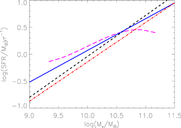
Figure 7. Comparison of the stellar mass and SFR relations for star-forming ETGs and composite ETGs. The black dashed line represents the best fit of Renzini & Peng (2015). The magenta long-dashed line shows the polynomial fit of all star-forming and composite galaxies (93,089 SFGs and 29,643 composite galaxies). Our result (the magenta line) is consistent with the finding of McPartland et al. (2019). The blue solid and red dotted–dashed lines are the fits for star-forming and composite ETGs, respectively (see the text).
Download figure:
Standard image High-resolution imageUsing 127,342 SFGs and 26,422 composite galaxies, McPartland et al. (2019) found that composite, Seyfert 2, and LINER galaxies can result in a "turnover" in the SFR and stellar mass relation for massive galaxies. In Figure 7, the magenta long-dashed line represents a polynomial fit of 122,732 galaxies, containing 93,089 SFGs and 29,673 composite galaxies located in the composite region of the [N II] BPT diagram. A total of 93,089 SFGs come from Wu (2020), and 29,673 composite galaxies are obtained by using the same method of Wu (2020). The fit is based on median values of 17 bins, 0.1 dex in mass; each bin includes more than 1100 galaxies. My fit is consistent with the result of McPartland et al. (2019) and this shows that these "non-star-forming" galaxies can influence measurements of the "main sequence." From Figure 7, we can see that star-forming and composite ETGs lie mainly on the "main sequence" (Noeske et al. 2007; Renzini & Peng 2015). This shows that the composite ETGs have lower SF activity than star-forming ETGs. Star-forming ETGs are compatible with the "main sequence" of SFGs, defined by star-forming galaxies at z ∼ 0 (Noeske et al. 2007; Schiminovich et al. 2007; Wuyts et al. 2011), while composite ETGs have ∼0.1 dex lower than star-forming ETGs. From Figures 4–7 and Table 1, we can reliably use the elliptical probability of p > 0.5 to derive the sample of ETGs and can compare their properties of star-forming and composite ETGs.
3.2. Comparison of Metallicity Properties for the Two Types of ETGs
In this section, we will utilize 4684 star-forming and 2011 composite ETGs dominated by SF to study their metallicities and to compare various properties. In this study, we use the metallicity indicator of Tremonti et al. (2004). In Wu (2020), the T04 method is a suitable metallicity estimator for composite ETGs, while the method is also used to estimate metallicity in star-forming ETGs (Wu et al. 2021, in preparation). Based on the T04 metallicity indicator of Wu (2020), composite ETGs have lower metallicity than SFGs, around 0.10 dex, at a fixed galaxy stellar mass. For the T04 indicator, star-forming ETGs have a median value of 12+log(O/H) ∼9.04, while composite ETGs present that of 12+log(O/H) ∼8.99. In ETGs, the dilution from gas inflow tends to decrease ≳0.2 dex in metallicity relative to the Tremonti et al. (2004) relation (Davis & Young 2019; Wu & Zhang 2021). Therefore, the metallicity difference is likely to come from the result of the dilution effect.
Figure 8(a), demonstrates the MZ relations for star-forming ETGs and composite ETGs with blue and red dots, respectively. The former ones do not significantly present a correlation between stellar mass and metallicity, with the Spearman coefficient r = 0.34, while the latter ones do not show a correlation between the two parameters, with the Spearman coefficient r = 0.17. Compared to the star-forming ETGs of Wu & Zhang (2021), our star-forming ETGs include some ETGs located in the composite and AGN regions of the [N II] BPT diagram, so our ETGs do not display a stronger correlation. Here, composite ETGs present a significantly weak correlation, and this is consistent with the result of Wu (2020), with other metallicity estimators. This may be due to external gas inflows into the ISM of galaxies, which dilutes their metallicities. As a result, the dilution effect may change their correlation.
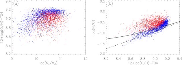
Figure 8. Comparison of MZ relations (left-hand panel) for star-forming and composite ETGs. Comparison of relations of 12+log(O/H) and log(N/O) (right-hand panel) for star-forming and composite ETGs. The black dashed line and solid curves are the secondary and primary+secondary relations in nitrogen production. The blue and red dots are the same as in Figure 1.
Download figure:
Standard image High-resolution imageSince star-forming ETGs and composite ETGs are dominated by the SF ionization source, we can introduce the N/O ratio to explore the relations between 12+log(O/H) and log(N/O) for the two types of ETGs. In Figure 8(b), we show relations between 12+log(O/H) and log(N/O) for star-forming and composite ETGs. The relations between two parameters present similar correlations and star-forming ETGs display the Spearman coefficient r = 0.48, while composite ETGs present a correlation, with the Spearman coefficient r = 0.45. From Figure 8(b), we can see that the star-forming ETGs include some ETGs with nitrogen-enriched H ii regions (Belfiore et al. 2015; Sánchez et al. 2015; Vincenzo et al. 2016), and therefore these star-forming ETGs do not have a significant correlation. According to the evolutionary schematic proposal of Garnett (1990) for N/O ratios, Coziol et al. (1999) presented a scheme that a sequence of SF bursts produce primary and secondary nitrogen in SFGs. Their nonlinear correlation derives from the combination of both nucleosyntheses (Mallery et al. 2007). The black curve and black dashed line represent, respectively, the primary+secondary and secondary relationship in nitrogen production. For primary nucleosynthesis, the N/O ratio will be generally constant, while the ratio has a linear correlation with 12+log(O/H) for second nucleosynthesis (Wu & Zhang 2013).
As can be seen from Figure 8(b), most star-forming ETGs lie in the black primary + secondary curve, while composite ETGs seem do not seem to be related to the black solid curve (the combination of both nucleosyntheses), although some of these ETGs lie on the curve. For composite ETGs, the nitrogen production is not likely to be explained by the evolutionary scheme proposed by Coziol et al. (1999). The model suggests that the N and O abundance increases in SFGs are due to these galaxies undergoing several SF processes in some cycles, and finally, the N/O ratio will increase to higher values. From Figures 10 and 11 of Wu & Zhang (2013), we can see that higher redshift or more massive galaxies often have statistically higher N/O abundance ratios, because the nitrogen enrichment of these galaxies have been started earlier (Wu & Zhang 2013). From the combination of Figures 8(a) and (b), we can see that Coziol et al. (1999)'s evolution scheme may explain the nitrogen production for star-forming ETGs of the [N II] BPT diagram, but the scheme cannot interpret the nitrogen production for these ETGs located in the composite and AGN regions of the [N II] BPT diagram. Although composite ETGs are dominated by SF, their nitrogen production may be derived from other nucleosyntheses.
For star-forming and composite ETGs, we describe their various comparisons. From Figure 5, star-forming and composite ETGs are located mainly at the GV region in the stellar mass and color diagram, and the two types of ETGs show that these ETGs are in a transition state. Considering their different SF activities (see Figures 4(b) and 7), their locations in the stellar mass and u − r color diagram, and their stellar masses of Figure 4(a), we may speculate that the two types of ETGs lie in a transition state, and they have experienced SF activities at a different time, but they are at different stages in a sequence of galaxy evolution: some star-forming ETGs have stronger SF activity, showing the properties of SFGs, while some composite ETGs do not present SF activity with significant properties of "dead" objects. In addition, Figure 8 shows that the two types of ETGs present different metallicities at a fixed stellar mass and have different nitrogen production schemes. We can see that the two types of ETGs had different excitation mechanisms in the past, although they now have the same SF excitation mechanism.
In the [N II] BPT diagram, galaxies located at the composite region may contain many ionization sources, such as shocks, cosmic rays, AGN activities, collisional excitation, and postasymptotic giant branch stars (Athey & Bregman 2009; Annibali et al. 2010; Griffith et al. 2019). In composite ETGs, their ionization mechanisms are likely to be the combination of more than one ionization source in the past, and these ETGs present an unordered nitrogen production state in Figure 8(b) before SF dominates their ionization emission mechanism. Because composite ETGs have probably many ionization sources, we cannot explore the nitrogen production on the 12+log(O/H) and log(N/O) diagram.
In Figure 9, I use the color bar of Dn 4000 to display the relations of 12+log(O/H) and log(N/O) for star-forming and composite ETGs. From Figure 9, we can see that these galaxies deviating from the primary+secondary relations for nitrogen production often present higher Dn 4000 values. This is consistent with the fact that a galaxy with older population central regions and no evidence of ongoing SF displays a larger deviation from the relation of 12+log(O/H) and log(N/O) of SFGs (Belfiore et al. 2015). In SFGs, the relation is related to the galaxy stellar mass, and more massive galaxies tend to have higher metallicities and higher N/O ratios (Wu & Zhang 2013). The nitrogen production is strongly associated with the history of the chemical evolution of a galaxy and nitrogen is primarily produced by intermediate-mass stars, so it has longer enrichment timescales relative to oxygen (Belfiore et al. 2015). We suggest that the inflowing scenario of metal-poor gas may explain the deviation from the relation of 12+log(O/H) and log(N/O). For these older massive ETGs with lower gas content, a small mass of pristine gas may dilute the metallicity considerably, but does not change the N/O abundance ratio significantly (Belfiore et al. 2015).

Figure 9. Comparison of relations of 12+log(O/H) and log(N/O) for star-forming ETGs (left-hand panel) and composite ETGs (right-hand panel) using the color bar of Dn 4000. The black dashed line and solid curves are the same as in Figure 8.
Download figure:
Standard image High-resolution imageIn addition, we investigate the correlation between sSFR and 12+log(O/H) in ETGs. Figure 10 displays the relations between sSFR and 12+log(O/H) for the two types of ETGs. The blue and red dots represent star-forming ETGs and composite ETGs, respectively. We find that the relation of sSFR and metallicity does not present a correlation for star-forming ETGs or composite ETGs, and the former ones have a Spearman coefficient r ∼ 0.14, while the latter ones present the Spearman coefficient r ∼ 0.24. When the two types of ETGs are combined, they also do not present a correlation with the Spearman coefficient r = 0.20.

Figure 10. Comparison of sSFR and 12+log(O/H) relations for star-forming and composite ETGs. The blue and red dots are the same as in Figure 1.
Download figure:
Standard image High-resolution image
Many studies explore the positive correlation and some explanations are proposed. Salim et al. (2014) deemed that the correlation is affected by some metallicity indicators. AGN feedback is considered by Lara-López et al. (2013) to cause the correlation, and they suggested that some galaxies have lower sSFR and metallicity, while other galaxies show higher sSFR and metallicity. Using different SFG samples from the SDSS data, the positive correlation is displayed at higher mass (e.g., Yates et al. 2012; Wu et al. 2019), showing the Spearman coefficient r = 0.44. From Figure 10, we can see that the positive correlation is not related to galaxy types, regardless of SFGs or ETGs. These results indicate that the positive correlation is likely to be in connection with the stellar mass.
4. Discussion
It is widely known that ETGs are "dead" objects, and are dominated by old stellar populations (Schlegel et al. 1998). By studying NUV photometry from the Galaxy Evolution Explorer (GALEX, Yi et al. 2005; Kaviraj et al. 2007) and statistical dissection of the optical spectra (Ferreras et al. 2006; Nolan et al. 2007; Rogers et al. 2007), it has been found that a large fraction of ETGs have experienced a small amount of recent SF (Rogers et al. 2009). ETGs that are still forming stars are an interesting class of objects. Why are they forming stars? In fact, ETGs are not as gas-poor as previously thought, and no less than 40% of low-redshift ETGs are now known to have molecular and/or atomic gas (Young et al. 2014).
The low-level SF of ETGs is attributed to two mechanisms suggested by many studies, internal and external. Internal mechanisms are an internal gas replenishment, which is an enriched material outflow from evolved stars joining the hot halo of the galaxy that may cool and fuel residual SF. External mechanisms include mergers and infall of low-metallicity gas. In the standard lambda cold dark matter (ΛCDM) universe, mergers play a crucial part in the assembly of galaxies (Van de Voort et al. 2018). Merger events tend to be divided into the two categories of minor mergers and major mergers; the former has more than one-fourth the mass ratio, while the latter has less than one-fourth. Each of the two types of mergers can be either gas-rich ("wet") or gas-poor ("dry;" van de Voort et al. 2018).
Although the cause of recent SF is uncertain, one possible scenario involves minor mergers. Minor mergers tend to contribute to low-efficiency SF in nearby ETGs, and Kaviraj (2014) found that at least ∼14% of the cosmic SF budget is supplied by this process. In ∼350 ETGs involving close pairs, Rogers et al. (2009) found that ETGs with close pairs enhance the level of recent SF relative to a control sample of ETGs. A strong correlation between UV color and the strength of the tidal distortions is demonstrated and Kaviraj (2010) suggested that the blue UV colors are driven by low-level merger-induced SF. In a sample of 67 ETGs, which are the most massive galaxies in the local universe, Davis et al. (2019) found that ∼22.4% of the sample have molecular gas content and suggested the supply of gas in these ETGs appears to be dominated by gas-rich mergers. Geré'b et al. (2016) found direct evidence for accretion in an extended stellar stream that extends ∼60 kpc beyond the galaxy center, which indicates that an ETG has experienced a minor merger in the past.
Another possible cause of recent SF may be related to inflow of the pristine material. NGC 4203 is a face-on ETG encircled by a large, low-column-density H i disk. Using infrared, deep-optical imaging, and UV data, Yildiz et al. (2015) studied the different components of the H i disk and found that the outer H i disk might be accreted from the metal-poor IGM. Salim et al. (2012) investigated 27 local ETGs with UV-detected SF and suggested that the gas-fueled current SFs of these ETGs has been accreted from the IGM. Concerning the formation of Hoag's Object, Finkelman et al. (2011) suggested that the core and H i disks of Hoag's Object were formed at different evolutionary phases, and that the forming of the disks was prolonged by "cold" accretion of pristine gas from the IGM.
In this work, I study the comparisons of various properties for the two types of ETGs and analyze mainly their primary+secondary production. For star-forming ETGs in the [N II] BPT diagram, we can use the evolution scheme of Coziol et al. (1999) to explain their nitrogen production. For some star-forming ETGs with composite and AGN regions located in the [N II] BPT diagram, we cannot interpret their nitrogen production by using the above-mentioned evolution scenario, and these ETGs do not comply with the primary+secondary production of SFGs. Regarding nitrogen production for the composite ETGs, we also need another mechanism to explain it.
Metallicity is one of the fundamental properties that describes the evolution of galaxies. In a large enough interstellar gas cloud, SF begins with the gravitational collapse of matter, and subsequent generations of stars are formed by using gas enriched by previous generations of stars. The outflow triggered by supernovae carries part of the gas, including heavy elements, out of the galaxy, while the inflow can bring pristine gas into the galaxy. The chemical enrichment can be interpreted by stellar metallicity throughout the SF history of the galaxy. Stellar metallicity is insusceptible to small variations in metallicity and gas-phase metallicity is sensitive to inflow and outflow (Coenda et al. 2020). Gallazzi et al. (2005) present that low-mass galaxies are young and stellar metal-poor, while high-mass galaxies are old and stellar metal-rich (Gallazzi et al. 2006), and they confirmed the good correlation between gas-phase metallicity and stellar metallicity by using galaxies with both measurements. Therefore, metallicity can trace the histories of SF and gas flows of galaxies (Fukagawa 2020). In light of this assumption, some studies explore the chemical evolution of these galaxies by comparing the gas-phase and stellar metallicities. Using a large sample of ETGs, Davis & Young (2019) found that some ETGs have lower gas-phase metallicities than their stellar metallicities and suggested that the gas fueling recent SF is accreted from an extra source. The metallicity decrease is attributed mainly to the dilution of galactic gas by infalling clouds (Westera et al. 2012).
Belfiore et al. (2015) utilized 14 MaNGA galaxies to study the relation between log(N/O) and 12+log(O/H) and found that at a given 12+log(O/H), some galaxies presented higher log(N/O) values, deviating from the contour for 50% of galaxies from the SDSS DR7. Infall of pristine gas may be a possible explanation, and it dilutes the metallicity, but it does not affect the N/O ratio significantly. In Figure 8, we can see that some star-forming ETGs, located in the composite and AGN regions of the [N II] BPT diagram, and most of the composite ETGs, deviate from the primary+secondary production of SFGs, and so we cannot use the evolution scenario of Coziol et al. (1999) to explain the nitrogen production of these ETGs. In fact, the relation between 12+log(O/H) and log(N/O) is related to stellar mass, and massive galaxies tend to present higher 12+log(O/H) and higher N/O values (Wu & Zhang 2013). Therefore, these massive galaxies are more evolved and dominated by secondary nitrogen production (Toloba et al. 2009) and by older intermediate-mass stars (Belfiore et al. 2015). In addition, I anticipate that the secondary nitrogen production increases with the galaxy stellar mass (Toloba et al. 2009). From Figure 9, most of these galaxies deviating from the primary+secondary nitrogen productions are older and more evolved, and present higher log(N/O) values. I suggest the outliers can be explained by low-metallicity inflow diluting the metallicities of these ETGs, while not significantly changing the log(N/O) values.
5. Summary
In this paper, I collect the observational data of 4684 star-forming ETGs and 2011 composite ETGs, which cross match the Galaxy Zoo 1 with the catalog of the SDSS DR7 MPA-JHU emission-line measurements. I compare the properties of both ETG samples and investigate their various properties. The main results are summarized as follows:
- 1.I present the distributions of stellar mass and sSFR for the two types of ETGs. Compared to star-forming ETGs, composite ETGs have higher stellar mass and lower sSFR.
- 2.In the stellar mass and color diagram, star-forming ETGs occupy the entire u − r color range, while composite ETGs take up mainly the GV and red sequence regions. More than 60% of star-forming and composite ETGs are located in the GV region.
- 3.In the WHAN diagram, all star-forming ETGs and most of the composite ETGs are located in the SF region, showing that these ETGs are dominated by SF. Compared with star-forming ETGs, composite ETGs have lower EWH α values.
- 4.I find that star-forming ETGs are located in the "main sequence" of SFGs, while composite ETGs lie below the "main sequence" of SFGs by about 0.1 dex. This indicates that the former ones have stronger SF activity than the latter ones.
- 5.On the basis of the above results, star-forming/composite ETGs mainly lie in a transition state and may have experienced SF activity at a different time. Compared with composite ETGs, star-forming ETGs had higher SF activity in the past, and perhaps composite ETGs experienced star formation even further in the past or more steadily/over longer timescales.
- 6.I demonstrate the MZ relations for star-forming and composite ETGs, with the Spearman coefficients r = 0.34 and r = 0.17, respectively. For composite ETGs, the poor correlation of the MZ relation may derive from the dilution result of gas inflow.
- 7.The relations between 12+log(O/H) and log(N/O) are described for both ETG samples, showing the Spearman coefficients r = 0.48 and r = 0.45 for star-forming and composite ETGs, respectively. From Figure 9, I suggest that nitrogen production for star-forming ETGs of the [N II] BPT diagram can be interpreted by Coziol et al. (1999)'s evolution scheme, while the production of composite ETGs (including some star-forming ETGs located in the composite and AGN regions of the [N II] BPT diagram) may be a sequence of the inflowing of metal-poor gas and in these more evolved massive galaxies.
- 8.The relations between sSFR and 12+log(O/H) for the two types of ETGs are displayed, showing a weaker correlation. According to related results, we suggest that the positive correlation is not related to galaxy types, and it is likely to be in connection with higher galaxy stellar mass.
Footnotes
- 1
- 2
- 3