


Abstract
The Andromeda galaxy (M31) is an object of ongoing study with the Ultraviolet Imaging Telescope (UVIT) on AstroSat. Field 2, which is 6.4 kpc in diameter at the distance of M31, includes a substantial part of the NE spiral arms of the galaxy. We have obtained a second observation of Field 2 with the far-ultraviolet (FUV) F148W (148 nm) filter, separated from the first observation by 1465 days. Both observations are analyzed to detect sources that are variable at a >3σ confidence level. For sources with less than ∼2'' separation, we apply multi-Gaussian fits, to obtain reliable magnitudes in the presence of source crowding. The variable sources are found to be concentrated in the spiral arms, with fraction of variable to nonvariable sources ∼2 times higher than for interarm regions, indicating an association of FUV variables with young stellar populations. UVIT FUV-NUV color–magnitude diagrams confirm the association of FUV variables with young massive/hot stars. Using existing catalogs, we obtain counterparts for 64 of the 82 most variable sources (>5σ). The counterparts include 13 star clusters, three ionized hydrogen (H ii) regions, three novae, one S Doradus star, eight eclipsing binaries, 20 foreground sources, two regular variables, and 14 unspecified variables.
Export citation and abstract BibTeX RIS
1. Introduction
The Andromeda galaxy (M31) is our closest neighboring giant spiral galaxy and has many similarities to our Galaxy. It can serve as a template for studies of parts of our Galaxy that are obscured by extinction. M31 has a well-measured distance (McConnachie et al. 2005) of 785 ± 25 kpc (3.2% error). The small distance uncertainty leads to well-measured luminosities for objects in M31.
M31 has been observed extensively in optical bands. The Hubble Space Telescope has yielded the highest resolution observations. These include the Panchromatic Hubble Andromeda Treasury (PHAT) survey (Williams et al. 2014). The GALEX instrument has observed M31 (Martin et al. 2005) in near- and far-ultraviolet (NUV and FUV) bands. More recently, M31 is part of an ongoing survey in NUV and FUV with the UltraViolet Imaging Telescope (UVIT) on AstroSat (Leahy et al. 2020).
The instruments onboard AstroSat include the following. The UVIT covers the FUV and NUV, while the Soft X-ray Telescope, Large Area Proportional Counters, Cadmium-Zinc-Telluride Imager, and Scanning Sky Monitor instruments cover soft through hard X-rays (Singh et al. 2014).
UVIT has a high spatial resolution (≃1''), which allows identifying individual stellar clusters and stars in M31. Leahy et al. (2021a) presents an analysis of the structure and stellar populations of the bulge. Leahy et al. (2021b) identifies FUV-variable sources in the central 28' of M31. Leahy et al. (2020) publishes the UVIT point-source catalog for M31. UVIT sources which match with Chandra sources in M31 are analyzed by Leahy & Chen (2020), and initial results of matching UVIT sources with PHAT sources are given by Leahy et al. (2021c). Leahy et al. (2018) analyze UV bright stars in the bulge, showing the existence of young stars in the bulge.
In this paper, we present results from two epochs of FUV observations in the 28' Field 2, NE of the bulge of M31. A new source-fitting algorithm that is suitable for regions with crowding is presented. We identify FUV-variable sources, and the population fractions of variable source numbers to nonvariable numbers are compared for different regions. Color–magnitude diagrams (CMDs) of variable and nonvariable sources are compared. Counterparts to >5σ variable are found using catalogs in the Vizier Web service, and NUV CMDs are used to investigate their nature. We close with a summary of the findings.
2. Observations and Data Analysis
UVIT observed M31 in FUV and NUV, covering the galaxy in nineteen 28' diameter fields (Leahy et al. 2020) with a ∼1'' spatial resolution. Tandon et al. (2017, 2020) give a detailed description of the UVIT instrument and its filters, which are labeled by their central wavelength in nm. UVIT Field 2 was observed in the F148W, F172M, N219M and N279N filters near the beginning of the observing project, in F172M in 2019, and in F148W in 2020. We call these three time periods Observation A, Observation B, and Observation C, respectively. The exposure times and dates of the observations for Field 2 are shown in Table 1.
Table 1. M31 UVIT Observations for UVIT Field 1
| Observation | Calendar Date | Mean BJD a | Filters b | Exposure Time (s) |
|---|---|---|---|---|
| A | 12-Nov-16 | 2457704.14 | F148W, N219M | 7942.8, 7986.2 |
| 2457704.49 | F172M, N279N | 7003.1, 7434.2 | ||
| B | 29-Oct-19 | 2458786.31 | F172M | 9353.2 |
| C | 14-15-Nov-20 c | 2459167.98 | F148W | 28395.1 |
Note.
a Mean Barycentric Julian Date of start of the observation. b For observation A, filter pairs F148W and N219M/ F172M and N279N were observed simultaneously. c Observation C had length of 1.28 days.Download table as: ASCIITypeset image
The F172M filter is narrow with δ λ = 12.5 nm versus 50 nm for F148W (Tandon et al. 2017), which results in a lower signal-to-noise ratio (S/N) than for the F148W images. As a result, only a fraction of the variables show up as variable above the >3σ level in F172M, and all of those are detected variables in F148W. The F172M filter in Observation B also has significant drift, which reduces the quality of the fits performed on the image. Thus, we use the F148W filter to create a catalog of variable sources for Field 2.
The data processing is carried out using the astrometry corrections given in Postma & Leahy (2020), and data processing and calibration methods given in Leahy et al. (2020).
2.1. Source Finding
The satellite pointing of AstroSat is dithered with the purpose of preventing burn out of individual channels in the microchannel plate electron multiplier of the UVIT detectors. The dither causes a low exposure time and consequently a high noise level at the edges of the UVIT field of view. Thus, we avoid the outer edge (∼1') for source finding (Leahy et al. 2021a).
Source finding is performed on the Field 2 F148W images using CCDLAB (Postma & Leahy 2017, 2021). For Observation A, the peak pixel S/N threshold is set to 4 and the threshold integrated S/N is set to 70. 1 For Observation C, the threshold peak pixel S/N is 5 and the threshold integrated S/N is 120. These different thresholds correspond to approximately the square root of the ratio of exposure times for the two images, which results in different sensitivities for the two images.
2.2. Source Magnitude Extraction
To determine the magnitude of the sources we use source fitting with elliptical Gaussians. An extra correction factor (Leahy et al. 2021b) is applied to account for the extended wings of the point-spread function (PSF), which extend out to ∼20'' (Tandon et al. 2017). This ensures that sources can be more accurately fit for M31, where there are few locations where sources are separated by ≳40'' (twice the PSF radius).
A source match is performed on the F148W filter source lists from Observations A and C using the TopCat catalog software (Taylor 2005). From this, 3793 sources are found to match to within one arcsecond between the two images. An additional 1392 sources are located in only Observation A and 1136 in only Observation C. For these sources, an upper limit on the magnitude is obtained in the corresponding location in the other image using CCDLAB. In total, this results in 6321 distinct sources. The positions of these sources are shown in Figure 1.

Figure 1. Field 2 with all identified UVIT sources from Observations A and C (gray crosses), >3σ variable sources (red circles), and >5σ variable sources (blue circles). There are 6231 total sources, 548 > 3σ variables, and 82 > 5σ variables.
Download figure:
Standard image High-resolution imageFor each source, the difference in flux between the two epochs and the error in the difference is calculated. Sources with a difference in magnitude more than three times the error are termed >3σ variables and sources with a difference more than five times the error are termed >5σ variables. A position is then calculated for each source based on a simple flux-weighted average of the two measurements. For Observation A, additional magnitudes are calculated in F172M, N219M, and N279N filters at this location. If the nearest light maxima in any of these filters is more than 1'' away, we list the filter magnitude as no detection since a position further than this likely corresponds to another source. We do not perform source fitting on the Observation B image because dithering-pointing errors during this observation made accurate photometry not possible. Overall, we obtain multiband magnitudes for most of the sources.
2.3. Identification of Variable Sources and Multi-Gaussian Fitting
The UVIT images of the >5σ variable sources are inspected to ensure that they are properly fit by CCDLAB's fitting program. Source positions that fell between two adjacent sources are removed from the totals of the sources listed above as are source centroids that are visibly off center for a source. We refit these sources using multi-Gaussian fitting, a newly programmed feature of CCDLAB created for this purpose.
Initial source position estimates and number of Gaussians, N, to use are determined by point-source extraction (PSE) centroiding. Each contributing Gaussian function is bounded in its position to ±1 pixel of the initial estimate. All contributing Gaussians share the same background, and the FWHMs of the major and minor axes of the elliptical Gaussian can be bounded to a common range input by the user. The Gaussian amplitudes are bounded between 0.5 and 2.0 times the initial estimate from the initial PSE centroiding. The general model equation for a Gaussian for N sources is shown in Equation 1, with an additional rotation transformation applied to allow for arbitrary orientation of the major axis of the elliptical Gaussian. The computational expense of fitting the compound elliptical Gaussian model increases rapidly with increasing N, and we generally limit such fits to N < 20.
Figures 2 and 3 show an examples of multi-Gaussian fits to two regions with sources for which single Gaussian fits result in poor photometry and source positions. The first case, which is fairly simple, has three sources with overlapping PSFs; and the second case, which is complex, has seven identifiable sources with overlapping PSFs.
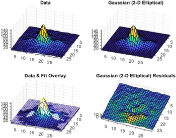
Figure 2. 3D plots for an example of a multi-Gaussian fit for a simple case of a single bright source with two nearby faint sources. The four panels show the data (upper left) for the 29 by 29 pixel image subarea which was fit, the three-Gaussian model (upper right), overlay of data and model (lower left), and residuals (lower right) that illustrate the success of the fit.
Download figure:
Standard image High-resolution image
Figure 3. 3D plots for an example of a multi-Gaussian fit for a complex case of several sources. The four panels show the data (upper left) for the 29 by 29 pixel image subarea that was fit, the seven-Gaussian model (upper right), overlay of data and model (lower left), and residuals (lower right) that illustrate the success of the fit.
Download figure:
Standard image High-resolution image61 of the >5σ sources are refit using multi-Gaussians in both observations A and C. This process yields 66 > 3σ sources including 16 > 5σ sources. For these sources, the listed R.A. and decl. is the average of the values in the two observations. 23 of the >3σ sources found through this method are ones previously detected with the individual fits. With this method we also find that five of the sources previously identified as >5σ variable are only variable at the >3σ level. Thus, we replace the individual fits for these sources with the multi-Gaussian fits as the multi-Gaussian fits give more reliable photometry and positions. In total, combining the sources which do not require multi-Gaussian fits and those that do, we obtain 548 > 3σ sources including 82 > 5σ variables.
2.4. A Test of the Statistics of Photometry Errors
We carried out a basic test on the measured flux differences for all detected F148W sources in Field 2. The absolute flux difference between the two epochs was divided by the flux error for each source to obtain a value greater than zero. This should have expected value ≃1 if the errors are estimated correctly. Figure 4 shows the distribution of these normalized flux differences. The mean and standard deviation of the normalized flux differences were calculated for two cases. Including all sources, the mean is 1.34 and standard deviation is 1.16; excluding the 548 > 3σ variable sources, the mean is 1.11 and standard deviation is 0.77. The latter group, which we label as nonvariable sources, is consistent with the expectation that the mean and standard deviation should be close to one.
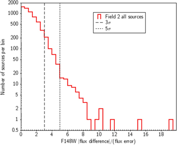
Figure 4. The distribution (red histogram) of the F148W flux differences, normalized to flux error of each source, for all Field 2 sources. The 3σ and 5σ lower limits for labeling a sources as >3σ or >5σ variable, are indicated. The nonvariable sources are taken as those with normalized flux difference <3.
Download figure:
Standard image High-resolution image2.5. Spatial Distribution of the Variable Sources
We check that the variable sources are not detected preferentially near the field edges. The radial distribution of source numbers versus distance from the mean field center (average of field centers of Observations A and C) is shown in Figure 5. The numbers of nonvariable sources per bin are multiplied by a factor of 0.1 so that the distribution of variables and nonvariables can be readily compared. Visually, they agree on large scale, within Poisson counting errors, with no peak at the field edge. The peak at about 0 15 corresponds to the radius that intersects the main spiral arm in Field 2 (SE spiral arm). This spiral arm also has a higher density of variable sources than other parts of the Field (Section 3.2), which accounts for the associated peak in variable sources. For the larger distance from the center (≳023), the number of variable sources drops off because the region selected for source fitting is elliptical in shape, causing the surveyed area to decrease.
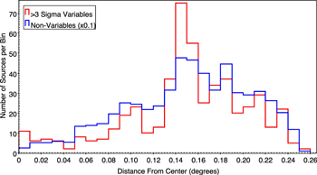
Figure 5. Numbers of variable and of nonvariable sources vs. distance from the field center.
Download figure:
Standard image High-resolution image2.6. Updates to Field 1
The UVIT observations of the central part of M31 (Field 1) are analyzed by Leahy et al. (2021a) to find FUV-variable sources. We reanalyze Field 1 by inspecting all >5σ sources and carrying out simultaneous multi-Gaussian fits to sources which have nearby sources (less than ∼2'' separation). The previous fits with single Gaussians in some cases give incorrect results, often because they choose an intermediate point between two or more sources for the fit. As a result, sources two, six, 29, and 34 from Table 4 of Leahy et al. (2021a) are not >5σ variables. One >3σ source is found to no longer be variable. One additional >5σ source and 5 additional >3σ sources are found using the multi-Gaussian fitting.
The majority of sources are not crowded (less than ∼2'' separation) and some that are crowded are fit correctly with single Gaussians. 2 Thus, we estimate ∼5% of the sources had unreliable photometry because of source crowding.
3. Results
3.1. Catalog of FUV Variables
Observation A has UVIT filters F148W, F172M, N219M, and N279N; Observation C has the F148W filter. Using the F148W photometry from Observations A and C, we create a catalog of the >3σ variables, which includes the >5σ variables. This catalog is presented here (first 10 entries) by Table 2, and in full as an online machine-readable table.
Table 2. Photometry a for >3σ Variable FUV Sources Measured in UVIT Field 2
| UVIT | UVIT | F148W_A | F148W_A | F148W_C | F148W_C | F148W | N279N_A | N279N_A | N219M_A | N219M_A | F172M_A | F172M_A |
|---|---|---|---|---|---|---|---|---|---|---|---|---|
| R. A. J2000 b | Decl. J2000 b | mag | err | mag | err | Sigma | mag | err | mag | err | mag | err |
| 10.97234 | 41.43923 | 20.57 | 0.06 | 32.05 | 5.42 | 19.16 | 18.62 | 0.05 | 19.87 | 0.08 | 20.65 | 0.14 |
| 10.98080 | 41.78037 | 20.17 | 0.05 | 23.66 | 0.12 | 15.46 | 20.48 | 0.11 | 20.69 | 0.11 | ⋯ | ⋯ |
| 11.22964 | 41.52613 | 19.59 | 0.04 | 18.73 | 0.04 | 11.89 | 18.78 | 0.06 | 18.03 | 0.05 | 18.60 | 0.07 |
| 11.17786 | 41.44147 | 19.42 | 0.04 | 20.32 | 0.04 | 10.48 | 19.50 | 0.08 | 19.53 | 0.07 | 19.89 | 0.10 |
| 11.20518 | 41.61675 | 20.91 | 0.07 | 22.67 | 0.08 | 10.04 | 20.58 | 0.12 | 21.11 | 0.13 | 22.03 | 0.25 |
| 11.23352 | 41.52304 | 18.43 | 0.03 | 18.92 | 0.04 | 9.66 | 18.29 | 0.05 | 18.49 | 0.05 | 18.80 | 0.07 |
| 11.08088 | 41.37964 | 20.62 | 0.06 | 21.91 | 0.06 | 8.92 | 18.60 | 0.05 | 21.55 | 0.16 | 21.00 | 0.16 |
| 11.04557 | 41.55410 | 18.21 | 0.03 | 18.60 | 0.04 | 8.29 | 17.42 | 0.04 | 17.70 | 0.04 | 18.05 | 0.06 |
| 11.15413 | 41.70736 | 22.18 | 0.11 | 25.69 | 0.29 | 8.15 | 19.62 | 0.08 | ⋯ | . | 21.67 | 0.21 |
| 10.87012 | 41.47448 | 20.71 | 0.06 | 19.75 | 0.04 | 8.11 | 19.42 | 0.07 | 19.20 | 0.06 | 19.59 | 0.09 |
Notes. Table 2 is published in its entirety in the machine-readable format. A portion is shown here for guidance regarding its form and content.
a Magnitudes are in the AB system; the value "." indicates no detection. b R.A. and decl. are measured in degrees.Only a portion of this table is shown here to demonstrate its form and content. A machine-readable version of the full table is available.
Download table as: DataTypeset image
3.2. Spatial Distribution of the FUV Variables
The comparison of all UVIT sources with the >3σ variable sources is given in Figure 1. The FUV-variable sources appear to be concentrated in the spiral arms in the east, center, and west parts of the image. A similar concentration of FUV-variable sources in spiral arms is found by Leahy et al. (2021a) for M31 Field 1 (their Figure 2).
Thus, we select arm and interarm regions on which to carry out statistical tests on the fraction of FUV variables. The new regions selected for Field 2 are shown with the previous regions selected for M31 Field 1 in Figure 6. Because we have a larger (continuous) view of the spiral arms, we change the names of the regions for Field 1 to more appropriate ones: SEarm is renamed E arm/F1; NEarm is now C arm/F1; ExtNWarm is now W arm/F1; ExtSEarm is now ExtE arm/F1; and ExtNEarm is now ExtC arm/F1. Thus, including both F2 and F1, the regions are E arm (blue in Figure 5), C arm (red), W arm (magenta and light magenta), ExtE arm (light blue), and ExtC arm (pink).

Figure 6. UVIT variable and nonvariable sources from Field 2 (upper left circle) and from Field 1 (lower right circle). For Field 2, the sources in the dense part of the east arm ("E arm") are shown in blue; those in the dense part of the central spiral arm ("C arm") in red; those in the west arm ("W-arm") in light magenta; and those not in any of the arms ("Interarm") in gray. For Field 1, the sources in the dense part of the east arm ("E arm") are shown in blue; those in the dense part of the central spiral arm ("C arm") in red; those in the dense part of the west arm ("W arm") in magenta. Sources in the intermediate density areas at southern part of E arm are shown in light blue ("ExtE arm"); and around the bulge ("ExtC arm") are shown in pink. Those in low-density regions/elsewhere ("Interarm") are shown in gray.
Download figure:
Standard image High-resolution image3.2.1. Distribution in Field 2
First consider the sources analyzed in Field 2. We compare the fractions of variable sources to all sources for the different regions. The polygon feature in TopCat is used to select four groups consisting of one for each of the dense parts of the east and central spiral arms (E arm and C arm), one for the right/west part of the image (W arm), and one for interarm sources (not in any of these regions). These groups are shown in the upper part of Figure 6 by blue, red, light-magenta, and gray circles, respectively.
Table 3 shows the results from counting sources from Field 2 in the different groups, with Poisson errors. In order, the C arm, E arm, W arm, and Interarm regions have decreasing fraction of variables. The fraction of variables is higher for the C arm than the Interarm by a factor of 2.7 and the E arm is higher than the Interarm by factor 1.7. Table 4 shows the significance of the differences by the difference of the ratios divided by the error in the difference (denoted by Σ). The C arm has a significantly higher fraction of variables than any of the other regions, and the E arm is significantly higher than Interarm.
Table 3. Field 2 Regions: Numbers of Sources, Variables, and Variable Fractions
| C arm | E arm | W arm | Interarm | |
|---|---|---|---|---|
| total number | 2022 | 1790 | 948 | 1512 |
| >3σ var. | 269 | 146 | 60 | 74 |
| >5σ var. | 48 | 16 | 8 | 10 |
| >3σ var./total | 0.1330 ± 0.0086 | 0.0810 ± 0.0070 | 0.0633 ± 0.0084 | 0.0489 ± 0.0058 |
| >5σ var./total | 0.0237 ± 0.0035 | 0.0089 ± 0.0022 | 0.0084 ± 0.0030 | 0.0066 ± 0.0021 |
Download table as: ASCIITypeset image
Table 4. Significance of Differences in >3σ Variable Fractions for Field 2 Regions
| C arm | E arm | W arm | Interarm | |
|---|---|---|---|---|
| C arm | n/a | |||
| E arm | 4.7Σ | n/a | ||
| W arm | 5.8Σ | 1.6Σ | n/a | |
| Interarm | 8.1Σ | 3.5Σ | 1.4Σ | n/a |
Note. The difference is given, in standard deviations, between the variable fraction for the region listed in column and the region listed in row.
Download table as: ASCIITypeset image
In summary, the C arm has the highest number and fraction of >3σ variables, and the E arm has a smaller excess of variables than either W-arm or Interarm regions. The majority of the >5σ variables (and highest fraction, see Table 3), are concentrated in the C arm.
3.2.2. Combined Distributions for Fields 1 and 2
A similar analysis of fraction of variable sources in Field 1 is carried out by Leahy et al. (2021a). We use these results but updated with the reanalysis of the photometry using multi-Gaussian fitting. The combined source lists of variable and nonvariable sources from Fields 1 and 2 are used to obtain statistics for the larger area covered by Fields 1 and 2.
The E-arm, ExtC-arm, C-arm, ExtC-arm, W-arm, and Interarm regions for Fields 1 and 2 are shown in Figure 6. Table 5 gives the resulting source numbers for these regions. 3 The Interarm region consists of the sources colored in gray in Figure 1. A new combined region, not ECarm, consists of all sources except those in the E arm and C arm.
Table 5. Fields 1 and 2 Combined: Numbers of Sources, Variables, and Variable Fractions
| C arm | E arm | W arm | Interarm | not ECarm | |
|---|---|---|---|---|---|
| total number | 3728 | 2732 | 1716 | 2562 | 5790 |
| >3σ var. | 458 | 250 | 108 | 220 | 402 |
| >5σ var. | 80 | 43 | 16 | 27 | 53 |
| >3σ var./total | 0.1229 ± 0.0061 | 0.0915 ± 0.0060 | 0.0629 ± 0.0062 | 0.0580 ± 0.0053 | 0.0694 ± 0.0036 |
| >5σ var./total | 0.0215 ± 0.0024 | 0.0157 ± 0.0024 | 0.0093 ± 0.0023 | 0.0078 ± 0.0019 | 0.0092 ± 0.0013 |
Download table as: ASCIITypeset image
The ratio of >3σ variables to all sources has the best statistics. Table 6 summarizes the significance of the differences in >3σ variable fractions between the different regions. The differences in fraction of variables between the C arm, E arm, and not ECarm are more significant for the >3σ variables than for >5σ variables. However the fractions have larger ratios between the different areas for the >5σ variables. Both lines of evidence show that the variable sources are more concentrated in the denser spiral arm regions than the nonvariable sources.
Table 6. Significance of Differences in >3σ Variable Fractions for Fields 1 and 2 Combined
| C arm | E arm | W arm | not ECarm | |
|---|---|---|---|---|
| C arm | n/a | |||
| E arm | 3.7Σ | n/a | ||
| W arm | 6.9Σ | 3.3Σ | n/a | |
| not ECarm | 7.6Σ | 3.1Σ | −0.9Σ | n/a |
Note. The difference is given, in standard deviations, between the variable fraction for the region listed in column and the region listed in row.
Download table as: ASCIITypeset image
In summary, the fractions of >3σ variables and >5σ variables in the C arm and E arm of Field 2 is similar to that for the C arm and E arm of Field 1, respectively. The C and E spiral arms have significantly higher fractions of variables than the rest of Fields 1 or 2.
3.3. Color–Magnitude Diagrams
We construct FUV-NUV CMDs for Observation A since it is the only observation with NUV filters. FUV is taken as F148W and NUV is taken as N279N. The CMD is shown in Figure 7 for all detected sources, 3–5σ variables and >5σ variables. On the CMDs, we show the isochrones of Bressan et al. (2012). 4 These isochrones use solar metallicity, a foreground extinction to M31 of AV = 0.2 and other parameters set to default in the isochrone generator.

Figure 7. Field 2 Observation A CMD: N279N vs. F148W-N279N. The gray points are all detected sources in Observation A, the black points are the >3σ variables, and the red points with error bars are the >5σ variables. The error bars for the gray and black points are similar in size, but not shown to avoid crowding. Isochrones are from Bressan et al. (2012), and are plotted as the points joined by solid lines, with log(age) values of 6.6 (blue lines), 7.1 (magenta lines), and 7.6 (cyan lines).
Download figure:
Standard image High-resolution imageThe majority of the objects in the CMD are placed between isochrones with ages ∼1.3 × 10⁷ yr to ∼4 × 10⁷ yr. Another significant fraction are in the area between the 4 × 10⁶ yr and 1.3 × 10⁷ yr isochrones. Because the observations select stars which are bright in the FUV and NUV bands, one expects a strong selection for the youngest stars in M31. A few of the data points (one variable and 25 nonvariables) are in the upper right area of the diagram, above the smallest age isochrone. We identify those as cool foreground stars in the Milky Way. If they were at the distance of M31 they would be shifted down by the difference in distance modulus (e.g., for a foreground stars at 1 kpc, the downward shift is 14.46 magnitudes). This shift moves those stars into the region consistent with isochrones with ages of a few Gyr, with N279N magnitudes ∼30.
3.4. Source Matching to Counterparts at Other Wavelengths
A search for counterparts is carried out for the set of 82 > 5σ FUV-variable sources. The online tool Vizier
5
(Ochsenbein et al. 2000) is used to find catalogs and sources that matched the UVIT FUV variables. The UVIT positions are good to <1'' (1σ error of 0 2), compared to a position accuracy of the counterparts, which is different for each catalog. The catalog position accuracies are typically ∼1'', so we use a search radius of 2'' from the UVIT positions to identify counterparts. Some counterparts are extended sources (stellar clusters), and these have a cluster effective radius, Reff, between 0.15 and 315. Reff is a factor in the choice of the 2'' search radius, so that we do not miss stellar clusters within which the UVIT source resides.
The counterpart search results are summarized in Table 7. Counterpart position, type, and distance from the UVIT position are listed. In cases where there is more than one counterpart we list them in order of the most-likely counterpart first and least-likely one last, with separation from the UVIT position and type of counterpart both factoring in our judgment of what is most likely. Twelve UVIT variable sources have three counterparts. 23 FUV variables have two listed counterparts, and the remaining 29 have one counterpart. The main categories of counterparts are 13 star clusters, three ionized hydrogen (H ii) regions, three novae, one S Doradus star, eight eclipsing binaries, 20 foreground sources, two regular variables, and 14 unspecified variables.
Table 7. Multiwavelength Counterparts of the UVIT FUV > 5σ VariablesA

|

| First catalog match | Separation | Reff | Distance[pc] | Second/third catalog match | Separation | Reff | Distance[pc] | |
|---|---|---|---|---|---|---|---|---|---|---|
| 11.08088 | 41.37964 | S Doradus Variable1 | 0.60 | Luminous Blue Variable14 | 0.37 | |||||
| Variable2 | 0.29 | |||||||||
| 11.13650 | 41.42231 | Cluster3 | 0.15 | 0.78 | H ii region15 | 0.81 | ||||
| Ionized nebula18 | 0.46 | |||||||||
| 11.00809 | 41.53676 | Variable2 | 0.25 | Periodic Variable4 | 0.75 | |||||
| Foreground Source9 | 0.25 | 1842 | ||||||||
| 11.29317 | 41.58330 | Variable2 | 0.18 | Cluster3 | 0.16 | 0.15 | ||||
| Foreground Source9 | 0.03 | 3382 | ||||||||
| 11.16057 | 41.41970 | Variable2 | 0.10 | Cluster16 | 0.98 | |||||
| Foreground Source9 | 0.16 | 4481 | ||||||||
| 11.02851 | 41.67441 | Eclipsing Binary4 | 0.89 | Cluster3 | 0.37 | 0.67 | ||||
| Foreground Source9 | 0.26 | 2712 | ||||||||
| 11.24051 | 41.52434 | H ii Region5 | 0.90 | Cluster3 | 1.26 | 1.78 | ||||
| Foreground Source9 | 0.42 | 3229 | ||||||||
| 10.86802 | 41.51010 | Variable2 | 0.26 | Variable17 | 0.09 | |||||
| Foreground Source9 | 0.30 | 2072 | ||||||||
| 11.25362 | 41.51686 | Cluster3 | 0.05 | 0.59 | Foreground source9 | 0.22 | 1172 | |||
| H ii Region14 | 0.26 | |||||||||
| 11.04513 | 41.53426 | Cluster3 | 0.03 | 0.81 | Globular cluster19 | 0.30 | ||||
| Hot Supergiant14 | 0.70 | |||||||||
| 11.00505 | 41.64860 | Eclipsing Binary4 | 0.29 | Variable17 | 0.42 | |||||
| Foreground source9 | 0.16 | 4790 | ||||||||
| 10.97206 | 41.77731 | Regular variable2 | 0.53 | Wolf-Rayet Star20 | 0.77 | |||||
| Foreground source9 | 0.49 | 2671 | ||||||||
| 11.15822 | 41.48995 | Eclipsing Binary2 | 0.32 | Foreground Source9 | 0.36 | 1429 | ||||
| 11.18793 | 41.44638 | Eclipsing Binary2 | 0.19 | Cluster3 | 0.18 | 3.15 | ||||
| 10.96305 | 41.41671 | Cluster3 | 0.81 | 1.53 | Foreground Source9 | 0.18 | 2475 | |||
| 11.22964 | 41.52613 | Variable2 | 0.39 | Foreground Source9 | 0.41 | 4234 | ||||
| 10.87012 | 41.47448 | Variable2 | 0.41 | Foreground Source9 | 0.28 | 2392 | ||||
| 11.20999 | 41.48600 | Eclipsing Binary2 | 0.39 | Foreground Source9 | 0.30 | 2039 | ||||
| 11.17494 | 41.44141 | H ii Region5 | 1.00 | Foreground Source9 | 0.75 | 3400 | ||||
| 11.08128 | 41.57281 | Variable2 | 0.52 | Foreground Source9 | 0.52 | 2974 | ||||
| 11.30144 | 41.62475 | Variable2 | 0.12 | Foreground Source9 | 0.17 | 1689 | ||||
| 11.30207 | 41.62134 | Cluster3 | 0.18 | 1.53 | Foreground Source9 | 0.40 | 2112 | |||
| 11.03645 | 41.52836 | H ii Region6 | 0.80 | Foreground Source9 | 0.47 | 3875 | ||||
| 11.23208 | 41.52771 | Variable2 | 0.46 | Foreground Source9 | 0.17 | 740 | ||||
| 11.18103 | 41.43686 | Variable2 | 0.95 | Foreground Source9 | 0.14 | 1477 | ||||
| 10.97973 | 41.41574 | Eclipsing Binary2 | 0.23 | Foreground Source9 | 0.24 | 4499 | ||||
| 11.14994 | 41.48801 | Cluster3 | 0.439 | 1.04 | Foreground Source9 | 0.79 | 2088 | |||
| 10.96437 | 41.42883 | Dubious Variable7 | 0.34 | Foreground Source9 | 0.34 | 15834 | ||||
| 11.31836 | 41.61420 | Variable2 | 0.83 | Foreground Source9 | 0.72 | 2100 | ||||
| 11.14319 | 41.40184 | Variable2 | 0.20 | Foreground Source9 | 0.22 | 1509 | ||||
| 11.20526 | 41.49038 | Cluster8 | 0.38 | Foreground Source9 | 0.28 | 1282 | ||||
| 11.26639 | 41.61990 | Cluster3 | 0.26 | 0.71 | Foreground source9 | 0.452 | 921 | |||
| 11.21039 | 41.48875 | Regular Variable2 | 0.44 | Foreground source9 | 0.52 | 6011 | ||||
| 11.18291 | 41.44354 | Cluster3 | 1.03 | 3.62 | Foreground source9 | 0.50 | 2031 | |||
| 11.18133 | 41.44383 | Cluster3 | 0.28 | 0.66 | Foreground source9 | 0.31 | 2966 | |||
| 11.17786 | 41.44147 | Foreground Source9 | 0.02 | 1319 | ||||||
| 11.23352 | 41.52304 | Foreground Source9 | 0.29 | 2171 | ||||||
| 11.04557 | 41.55410 | Foreground Source9 | 0.34 | 5035 | ||||||
| 11.10292 | 41.59112 | Foreground Source9 | 0.28 | 2977 | ||||||
| 11.31195 | 41.63195 | Foreground Source9 | 0.04 | 1158 | ||||||
| 11.30086 | 41.65048 | Variable10 | 0.71 | |||||||
| 11.23841 | 41.52736 | Eclipsing Binary2 | 0.24 | |||||||
| 11.02351 | 41.64972 | Cluster3 | 0.11 | 0.57 | ||||||
| 11.21590 | 41.48749 | Foreground Source9 | 0.41 | 2599 | ||||||
| 11.29147 | 41.61409 | Foreground Source9 | 0.35 | 1297 | ||||||
| 11.22379 | 41.60010 | Variable2 | 0.08 | |||||||
| 11.14180 | 41.41971 | Cluster3 | 0.32 | 0.17 | ||||||
| 11.27372 | 41.62386 | Eclipsing Binary2 | 0.82 | |||||||
| 11.02500 | 41.64983 | Cluster3 | 0.45 | 0.21 | ||||||
| 10.79765 | 41.60537 | Foreground Source9 | 0.66 | 505 | ||||||
| 10.97234 | 41.43923 | Nova11 | 0.86 | |||||||
| 11.15413 | 41.70736 | Nova12 | 0.44 | |||||||
| 11.07571 | 41.54640 | Nova13 | 0.91 | |||||||
| 10.98080 | 41.78037 | Foreground Source9 | 0.24 | 3952 | ||||||
| 11.20518 | 41.61675 | Foreground Source9 | 0.45 | 1563 | ||||||
| 11.19808 | 41.47936 | Foreground Source9 | 0.60 | 1953 | ||||||
| 11.19912 | 41.47905 | Foreground Source9 | 0.20 | 3506 | ||||||
| 11.21058 | 41.48442 | Foreground Source9 | 0.22 | 807 | ||||||
| 10.76520 | 41.60412 | Foreground Source9 | 0.49 | 2137 | ||||||
| 10.96876 | 41.78298 | Foreground Source9 | 0.27 | 2079 | ||||||
| 11.15802 | 41.42109 | Foreground Source9 | 0.44 | 6587 | ||||||
| 11.23510 | 41.52603 | Foreground Source9 | 0.48 | 1953 | ||||||
| 11.17610 | 41.44080 | Foreground source9 | 0.87 | 2265 | ||||||
| 10.98125 | 41.78141 | Foreground source9 | 0.46 | 7321 |
Note. A: R.A. and decl. are sky position of the UVIT FUV variable in decimal degrees. The first, second, and third catalog matches refer to the identified typing of the object in catalogs in Vizier. Distance refers to the separation in arcseconds between the UVIT source and the identified match from Vizier. Reff gives the radius of the cluster from the literature for sources that match with a cluster. Catalog references: Samus' et al. (2017), Vilardell et al. (2006), Johnson et al. (2015), Bonanos et al. (2003), Hodge et al. (2011), Azimlu et al. (2011), Heinze et al. (2018), Williams & Hodge (2001), Bailer-Jones et al. (2021), Bonanos et al. (2019), Hornoch & Kucakova (2016), Darnley & Williams (2016), Williams et al. (2019), Humphreys et al. (2017), Lee & Lee (2014), Kang et al. (2012), An et al. (2004), Walterbos & Braun (1992), Peacock et al. (2010), Neugent et al. (2012).
We use the Gaia (Gaia Collaboration et al. 2016, 2018; Gaia Collaboration 2018) EDR3 to determine foreground counterparts and included those sources where a distance, "rgeo," is provided in Bailer-Jones et al. (2021). This provides many more foreground counterparts for Field 2 than we found for Field 1 (Leahy et al. 2021a). Many of the UVIT variables with foreground counterparts for Field 2 also have a variable star in M31 as counterpart. In these cases, the known variable is the probable real counterpart. For the remaining cases with two or more counterparts (none a foreground star), most likely the counterparts from different catalogs are the same object or correspond to bright objects inside clusters or H ii regions.
We found that 64 of the 82 UVIT FUV > 5σ variables match sources at other wavelengths. The majority of the matches are with objects associated with variability. The UVIT CMDs for the FUV > 5σ variables is shown in Figure 8. The counterpart types are labeled using the First Catalog Match from Table 7. Because a given counterpart may not have a N279N measurement or may be too faint in N279N, not all 64 counterparts are visible on the CMD.

Figure 8. Field 2 Observation A CMD with N279N versus F148W-N279N. The gray points with error bars are the FUV > 5σ variable source measurements from Observation A, and the red symbols mark the identified counterparts from Table 7. Isochrones are from Bressan et al. (2012), and are plotted as the points joined by solid lines, with log(age) values of 6.6 (blue lines), 7.1 (magenta lines), and 7.6 (cyan lines).
Download figure:
Standard image High-resolution imageThe brightest FUV variables, above the 1.3 × 10⁷ yr isochrone in Figure 8, are identified as hot supergiants or residing in clusters or H ii regions. This is consistent with their locations in the CMD. The S Doradus star has F148W magnitudes in Observations (A, C) of (20.62, 21.91). This is a significant difference (1.29 magnitudes) compared to the small error of ∼0.06 magnitudes. The FUV variables intermediate in luminosity, near the 1.3 × 10⁷ yr isochrone, are mostly variables of unknown types as well as clusters, H ii regions and some eclipsing binaries. The majority of the sources that match with foreground sources are also at this brightness, with the exception of the bright foreground source in the upper-right corner of the CMD. This source has a F148W magnitude change of 20.40–21.02 between Observations A and C and a very bright N279N magnitude of 15.45. As such, it very likely corresponds to the foreground source at a distance of 505 pc (Bailer-Jones et al. 2021). The fainter FUV variables, near the 4 × 10⁷ yr isochrone, are identified with the eclipsing binaries and variables of unknown type.
A sample (the first 10 lines) of the UVIT FUV-variable source catalog is given here in Table 2. The full catalog is available as an online Table, for the purpose of allowing further investigations of individual sources.
3.5. Comparison with Field 1
Figure 9 shows the CMD for the >5σ UVIT counterparts from both Field 2 (current work) and Field 1 (Leahy et al. 2021a; with the updated list of FUV variables as noted in Section 2.6). Field 2 has more counterparts than Field 1 corresponding to eclipsing binaries. It has fewer novae and variables with a regular or semiregular periodicity.

Figure 9. Idem Figure 8, for Fields 1 and 2.
Download figure:
Standard image High-resolution image
4. Summary and Conclusion
We carry out a new observation of Field 2 of M31 such that Field 2 has been observed in the F148W filter at two epochs separated by ≃4 yr. Field 2 is a 28' diameter (6.4 kpc) circular region, which covers a significant part of the spiral arms in the NE part of M31.
New multi-Gaussian fitting capability in the CCDLAB analysis software enables source photometry in crowded regions. With the two epochs of F148W photometry, we identify FUV-variable sources. A total of 3793 sources are detected in both Observations A and C, 1392 are only detected in A, and 1136 are only detected in C. From this set of 6321 sources, 548 (≃8%) are found to be variable by >3σ and 82 (≃1%) are found variable by >5σ.
The UVIT F148W filter (148 nm band) is sensitive to detection of hot luminous stars. The current analysis shows that the fraction of variable sources is higher, by factor of ∼2, in the regions (E and C spiral arms in Field 2) with the highest hot-star density compared to the regions with lowest density (Interarm) or regions with intermediate density (e.g. W arm). The regions with the lowest density and with a medium density of young hot stars have similar fractions of variable stars (<1 standard deviation difference). Thus most variables are associated with young stellar systems concentrated in the dense parts of the spiral arms.
Counterparts for the FUV-variable sources are found. A wide variety of types are identified, and most are associated with previously identified young hot variable stars (see Table 7). Of the 82 sources, 64 match to a previously known source. Most of these are known optical variable sources. The main categories include star clusters, eclipsing binaries, H ii regions, nova or nova candidates, an S Doradus star, and other variables.
The CMD for Observation A (Figure 7) shows that most FUV-variable sources are consistent with young stars. The range of inferred ages for the FUV variables is ∼5 × 10⁶ yr to ∼1 × 10⁸ yr. The variable stars, in comparison to the nonvariable stars are concentrated higher up in the CMD (brighter N279N magnitudes), where younger stars are located, based on the isochrones. This confirms that the majority of variable stars are associated with young stars. This is consistent with the results from the spatial analysis which associates most FUV variables with the spiral arms.
The FUV-variable sources from Field 2 are combined with those from the those for the central part (Field 1) of M31 (Leahy et al. 2021a). The combined spatial analysis (Table 5) gives results consistent with that for Field 1 (the fraction of variables is ∼2 times higher for spiral arms than interarm regions), but with much better statistics. The combined NUV-FUV CMD of the UVIT variables and their counterparts from Fields 1 and 2 (Figure 9) confirms the association of most FUV variables with young hot stars.
The catalog of the UVIT FUV variables for Field 2 is made available online with this paper, with aim to facilitate future multiwavelength research of individual objects of interest.
This work is supported by funding from the Canadian Space Agency, and the Natural Sciences and Engineering Research Council of Canada. This publication uses data from the AstroSat mission of the Indian Space Research Institute (ISRO), archived at the Indian Space Science Data Center (ISSDC). This work has made use of data from the European Space Agency (ESA) mission Gaia (https://www.cosmos.esa.int/gaia), processed by the Gaia Data Processing and Analysis Consortium (DPAC; https://www.cosmos.esa.int/web/gaia/dpac/consortium). Funding for the DPAC has been provided by national institutions, in particular the institutions participating in the Gaia Multilateral Agreement. We thank the anonymous referee for comments which lead to several improvements in this article.
Footnotes
- 1
Threshold integrated S/N is the minimum ratio of (detected counts above background summed over pixels in the detection window) to (background counts summed over pixels in the window).
- 2
Likely because the fainter source was much less bright.
- 3
ExtE arm and ExtC arm, which are only in Field 1, are given in Leahy et al. (2021a) with names ExtSEarm and ExtNEarm.
- 4
Calculated using the CMD web isochrone generator at http://stev.oapd.inaf.it/cmd.
- 5